nenupy.instru.nenufar.MiniArray
- class nenupy.instru.nenufar.MiniArray(index=0, antenna_delays=None, antenna_weights=None, use_generic_antenna_model=True)[source]
Bases:
InterferometerMain class to handle a NenuFAR Mini-Array antenna distribution.
Added in version 2.0.0.
- Parameters:
index (
int) – Mini-Array index. ‘Core’ Mini-Arrays have indices ranging from0to95. ‘Remote’ Mini-Arrays have indices ranging from100to105.- Example:
Instantiating
MiniArray:>>> from nenupy.instru import MiniArray >>> ma = MiniArray(index=0)
Sub-arraying on an existing
MiniArrayinstance:>>> sub_ma = ma["Ant01", "Ant06", "Ant11"] >>> sub_ma.antenna_names array(['Ant01', 'Ant06', 'Ant11'], dtype='<U5')
Using
sliceobject (converted inndarrayusingr_):>>> import numpy as np >>> sub_ma = ma[np.r_[2:10]] >>> sub_ma.size 8
Combining two
MiniArrayinstances:>>> ma1 = MiniArray(index=0)["Ant01", "Ant06"] >>> ma2 = MiniArray(index=0)["Ant08", "Ant12"] >>> combined_ma = ma1 + ma2 >>> combined_ma.antenna_names array(['Ant01', 'Ant06', 'Ant08', 'Ant12'], dtype='<U5')
See also
More details on this class usage can be found in Array Configuration and Instrument Properties.
Attributes Summary
Mini-Array index.
Mini-Array rotation.
Array's position.
Antenna names.
Antenna positions.
Antenna gains.
Instrument baselines.
Number of elements belonging to the array.
antenna_weightsAdd delay errors for each antennae They could be cable connection errors during construction, cables of wrong length, ...
Methods Summary
beam([sky, pointing, configuration, ...])Computes the Mini-Array beam over the
skyfor a givenpointing.effective_area([frequency, elevation])Computes the effective area of a NenuFAR Mini-Array.
instrument_temperature([frequency, lna_filter])Instrument temperature at a given
frequency.attenuation_from_zenith(coordinates[, time, ...])Returns the attenuation factor evaluated at given
coordinatescompared to the zenithal Mini-Array beam gain.analog_pointing(pointing, configuration)Converts the desired pointing to the effective pointing which depends on the available pointing positions defined on a grid due to analog cable delays.
beamsquint_correction(coords[, frequency])Corrects for the beamsquint effect.
plot(**kwargs)Plots the antenna distribution.
array_factor(sky, pointing[, ...])Computes the array factor of the antenna distribution.
system_temperature([frequency, ...])Computes the System Noise Temperature \(T_{\rm sys}\).
sefd([frequency, elevation, efficiency, ...])Computes the System Equivalent Flux Density (SEFD or system sensitivity).
sensitivity([frequency, mode, dt, df, ...])Computes the sensititivy of the array with respect to the observing configuration.
angular_resolution([frequency])Computes the angular resolution of the antenna array.
confusion_noise([frequency, lofar])Confusion rms noise \(\sigma_{\rm c}\) (parameter used for specifying the width of the confusion distribution) computed as:
Attributes and Methods Documentation
- __init__(index=0, antenna_delays=None, antenna_weights=None, use_generic_antenna_model=True)[source]
Methods
__init__([index, antenna_delays, ...])analog_pointing(pointing, configuration)Converts the desired pointing to the effective pointing which depends on the available pointing positions defined on a grid due to analog cable delays.
angular_resolution([frequency])Computes the angular resolution of the antenna array.
array_factor(sky, pointing[, ...])Computes the array factor of the antenna distribution.
attenuation_from_zenith(coordinates[, time, ...])Returns the attenuation factor evaluated at given
coordinatescompared to the zenithal Mini-Array beam gain.beam([sky, pointing, configuration, ...])Computes the Mini-Array beam over the
skyfor a givenpointing.beamsquint_correction(coords[, frequency])Corrects for the beamsquint effect.
confusion_noise([frequency, lofar])Confusion rms noise \(\sigma_{\rm c}\) (parameter used for specifying the width of the confusion distribution) computed as:
effective_area([frequency, elevation])Computes the effective area of a NenuFAR Mini-Array.
instrument_temperature([frequency, lna_filter])Instrument temperature at a given
frequency.plot(**kwargs)Plots the antenna distribution.
sefd([frequency, elevation, efficiency, ...])Computes the System Equivalent Flux Density (SEFD or system sensitivity).
sensitivity([frequency, mode, dt, df, ...])Computes the sensititivy of the array with respect to the observing configuration.
system_temperature([frequency, ...])Computes the System Noise Temperature \(T_{\rm sys}\).
Attributes
Add delay errors for each antennae They could be cable connection errors during construction, cables of wrong length, ...
Antenna gains.
Antenna names.
Antenna positions.
antenna_weightsInstrument baselines.
Mini-Array index.
Array's position.
Mini-Array rotation.
Number of elements belonging to the array.
- analog_pointing(pointing, configuration)[source]
Converts the desired pointing to the effective pointing which depends on the available pointing positions defined on a grid due to analog cable delays.
- angular_resolution(frequency=<Quantity 50. MHz>)
Computes the angular resolution of the antenna array.
The full width at half maximum (FWHM) \(\theta\) is approximated as follows:
\[\theta = \frac{\lambda}{D}\]where \(\lambda\) is the wavelength and \(D\) is is the length of the maximum physical separation of the antennas in the array.
- property antenna_delays
Add delay errors for each antennae They could be cable connection errors during construction, cables of wrong length, …
- property antenna_gains
Antenna gains. This is an array of
callable(methods or functions) defining the radiation pattern of each antenna.
- property antenna_names
Antenna names.
- Setter:
Array of antenna names.
- Getter:
Array of antenna names.
- Type:
- property antenna_positions
Antenna positions. The positions should be shaped as
(n_ant, 3)- Setter:
Array of antenna positions.
- Getter:
Array of antenna positions.
- Type:
- array_factor(sky, pointing, return_complex=False, normalize=True)
Computes the array factor of the antenna distribution.
\[\mathcal{F}(\nu, \phi, \theta) = \sum_{\rm ant} w_{\rm ant} e^{ i \mathbf{k}(\nu, \phi, \theta) \cdot \mathbf{r}_{\rm ant}}\]where \(\mathbf{k} = \frac{2\pi}{\lambda} (\cos \phi \cos \theta, \sin \phi \cos \theta, \sin \theta )\) is the wave vector for a wave propagation in a direction described by spherical coordinates, \(\lambda\) is the wavelength, \(\phi\) is the azimuth, \(\theta\) is the elevation, \(\mathbf{r}_{\rm ant}\) is the antenna position matrix, \(w_{\rm ant}\) is the weight of the antenna (defined in
feed_weights).This method considers the
skyas the desired output (in terms of time, frequency and sky positions). It evaluates the effective pointing directions for every time step defined inskyregarding thepointinginput.- Parameters:
sky (
Sky) – Desired output contained in aSkyinstance. (time,frequencyandcoordinatesare used as inputs for the computation).pointing (
Pointing) – Instance ofPointingthat defines the targeted pointing directions over the time.return_complex (
bool) – Return complex array factor ifTrueor power ifFalsenormalize (
bool) – Return the normalized array factor. Default isTrue.
- Returns:
Array factor of the antenna distribution shaped as
(time, frequency, 1, coordinates).- Return type:
- attenuation_from_zenith(coordinates, time=<Time object: scale='utc' format='datetime' value=2026-07-06 12:39:54.157713>, frequency=<Quantity 50. MHz>, polarization=Polarization.NW)[source]
Returns the attenuation factor evaluated at given
coordinatescompared to the zenithal Mini-Array beam gain.- Parameters:
coordinates (
SkyCoord) – Sky positions equatorial coordinates.time (
Time) – UTC time at which the attenuation is evaluated. Default isnow.frequency – Frequency at which the attenuation is evaluated. Default is
50 MHz.polarization (
Polarization) – NenuFAR antenna polarization. Default isPolarization.NW.
- Returns:
Attenuation factor shaped as
(time, frequency, polarization, coordinates).NaNis returned for anycoordinatesthat is below the horizon.- Return type:
- Example:
>>> from nenupy.instru.nenufar import MiniArray
>>> from astropy.coordinates import SkyCoord
>>> ma = MiniArray(index=0)
>>> attenuation = ma.attenuation_from_zenith(
        coordinates=SkyCoord.from_name("Cyg A")
    )
>>> from nenupy.instru.nenufar import MiniArray
>>> from astropy.coordinates import SkyCoord
>>> import astropy.units as u
>>> ma = MiniArray(index=0)
>>> attenuation = ma.attenuation_from_zenith(
        coordinates=SkyCoord.from_name("Cyg A"),
        frequency=np.linspace(20, 80, 10)*u.MHz
    )
Added in version 2.0.0.
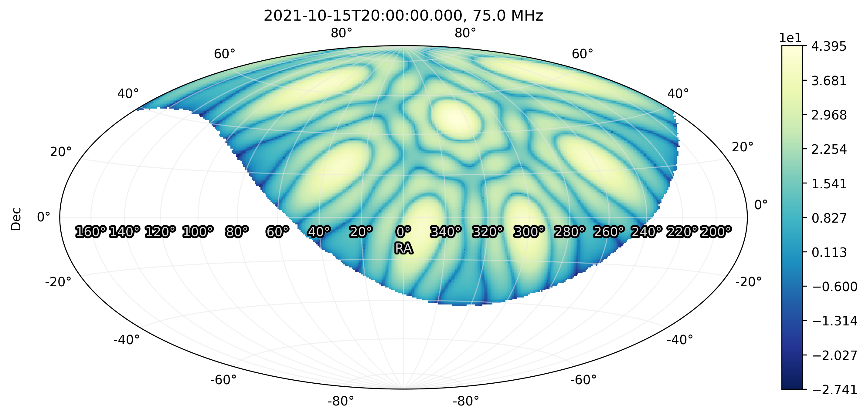
- beam(sky=<nenupy.astro.sky.HpxSky object>, pointing=<nenupy.astro.pointing.Pointing object>, configuration=<nenupy.instru.nenufar.NenuFAR_Configuration object>, return_complex=False, normalize=True)[source]
Computes the Mini-Array beam over the
skyfor a givenpointing.\[\mathcal{G}_{\rm MA}(\nu, \phi, \theta) = \mathcal{F}_{\rm MA}(\nu, \phi, \theta) \mathcal{G}_{\rm ant} (\nu, \phi, \theta)\]where \(\nu\) is the frequency, \(\phi\) is the azimuth, \(\theta\) is the elevation, \(\mathcal{G}_{\rm ant}\) is the NenuFAR dipole antenna radiation pattern and \(\mathcal{F}_{\rm MA}\) is the array factor.
This method considers the
skyas the desired output (in terms of time, frequency, polarization and sky positions). It evaluates the effective pointing directions for every time step defined inskyregarding thepointinginput.- Parameters:
sky (
Sky) – Desired output contained in aSkyinstance. (time,frequency,polarizationandcoordinatesare used as inputs for the computation).pointing (
Pointing) – Instance ofPointingthat defines the targeted pointing directions over the time.configuration (
NenuFAR_Configuration) – NenuFAR configuration to consider during the beam simulation. The beamsquint correction and its frequency setting are defined here. Default isNenuFAR_Configuration(beamsquint_correction=True, beamsquint_frequency=50MHz).
- Returns:
The instance of
Skygiven as input is returned, its attributevalueis updated with the result of the beam computation (stored as anArray) and shaped as(time, frequency, polarization, coordinates).- Return type:
- Example:
Load the required librairies:
>>> from nenupy.instru import MiniArray, Polarization
>>> from nenupy.astro.sky import HpxSky
>>> from nenupy.astro.pointing import Pointing
>>> import astropy.units as u
>>> from astropy.time import Time, TimeDelta
Define a desired
Skyoutput:>>> sky = HpxSky( resolution=1.*u.deg, frequency=np.array([25, 50, 75])*u.MHz, polarization=np.array([Polarization.NW, Polarization.NE]), time=Time("2021-10-15 20:00:00") )
Define the pointing of the Mini-Array:
>>> ma_pointing = Pointing.zenith_tracking(
        time=Time("2021-10-15 00:00:00"),
        duration=TimeDelta(3600*24, format="sec")
    )
Select the Mini-Array (and possibly its antenna distribution) and compute its response pattern:
>>> ma = MiniArray(1)
>>> beam = ma.beam(
        sky=sky,
        pointing=ma_pointing
    )
Calling
print()on aSkyobject enables the display of itsvalueattribute structure (which matches the definition of theskyinstance):>>> print(beam) <class 'nenupy.astro.sky.HpxSky'> instance value: (1, 3, 2, 49152) * time: (1,) * frequency: (3,) * polarization: (2,) * coordinates: (49152,)
To
plot()the computed Mini-Array response at 75 MHz, in NE polarization:>>> beam[0, 2, 1].plot( decibel=True, colorbar_label='' )
See also
- beamsquint_correction(coords, frequency=<Quantity 50. MHz>)[source]
Corrects for the beamsquint effect.
- Example:
>>> from astropy.coordinates import SkyCoord, AltAz
>>> from astropy.time import Time
>>> import astropy.units as u
>>> from nenupy import nenufar_position
>>> from nenupy.instru import MiniArray
>>> position = SkyCoord(
        0*u.deg,
        30*u.deg,
        frame=AltAz(
            obstime=Time("2021-01-01 12:00:00"),
            location=nenufar_position
        )
    )
>>> ma = MiniArray()
>>> corrected_position = ma.beamsquint_correction(
        coords=position,
        frequency=50*u.MHz
    )
>>> corrected_position.az.deg, corrected_position.alt.deg
(0., 22.91422672)
- confusion_noise(frequency=<Quantity 50. MHz>, lofar=True)
Confusion rms noise \(\sigma_{\rm c}\) (parameter used for specifying the width of the confusion distribution) computed as:
\[\left( \frac{\sigma_{\rm c}}{\rm{mJy}\, \rm{beam}^{-1}} \right) \simeq 0.2 \left( \frac{\nu}{\rm GHz} \right)^{-0.7} \left( \frac{\theta}{\rm arcmin} \right)^{2}\]or (if
lofar=True):\[\left( \frac{\sigma_{\rm c}}{\mu\rm{Jy}\, \rm{beam}^{-1}} \right) \simeq 30 \left( \frac{\nu}{74 {\rm MHz}} \right)^{-0.7} \left( \frac{\theta}{\rm arcsec} \right)^{1.54}\]where \(\nu\) is the frequency and \(\theta\) is the radiotelescope FWHM (see
angular_resolution()).Individual sources fainter than about \(5\sigma_{\rm c}\) cannot be detected reliably.
- Parameters:
freq (
floatorQuantity) – Frequency at which computing the confusion noise. In MHz if no unit is provided. Default is50 MHz.miniarrays (
int,listorndarray) – Mini-Array indices to take into account. Default isNone(all available MAs).lofar – If set to
True(recommended), the confusion noise is estimated using Eq. 6 of van Haarlem et al. (2013).
- Type:
- Returns:
Confusion rms noise in Jy/beam
- Return type:
- Example:
>>> import astropy.units as u
>>> <instrument>.confusion_noise(
        frequency=50*u.MHz
    )
- effective_area(frequency=<Quantity 50. MHz>, elevation=<Quantity 90. deg>)[source]
Computes the effective area of a NenuFAR Mini-Array. The effective area of a Mini-Array (\(\mathcal{A}_{\rm eff,\ MA}\)) is computed as the sum of dipole effective areas (\(\mathcal{A}_{\rm eff, ant}\)), while taking into account overlaps. This is a function of
frequency(\(\nu\)) andelevation(\(\theta\)):\[\mathcal{A}_{\rm eff,\ MA} (\nu) = \sum_{\rm ant} \mathcal{A}_{\rm eff, ant} (\nu) \sin( \theta )\]with
\[\mathcal{A}_{\rm eff, ant} (\nu) = \frac{\lambda^2}{3}\]the NenuFAR dipole antenna effective area.
- Parameters:
- Returns:
Effective area of a Mini-Array shaped as
frequency.- Return type:
- Example:
>>> from nenupy.instru import MiniArray
>>> import astropy.units as u
>>> ma = MiniArray()
>>> ma.effective_area(50*u.MHz)
227.68377 m2
>>> ma = MiniArray()
>>> ma.effective_area(frequency=50*u.MHz, elevation=45*u.deg)
160.99673 m2
>>> ma = MiniArray()["Ant01"]
>>> ma.effective_area(50*u.MHz)
11.979179 m2
>>> ma = MiniArray()
>>> ma.effective_area(u.Quantity([20, 30, 40], unit='MHz'))
[693.44216, 532.97815, 355.85306] m2
See also
- property index
Mini-Array index. ‘Core’ Mini-Arrays have indices ranging from
0to95. ‘Remote’ Mini-Arrays have indices ranging from100to105.- Setter:
Mini-Array index.
- Getter:
Mini-Array index.
- Type:
- static instrument_temperature(frequency=<Quantity 50. MHz>, lna_filter=0)[source]
Instrument temperature at a given
frequency. This depends on the Low Noise Amplifier characteristics.- Parameters:
frequency (
Quantity) – Frequency at which computing the instrument temperature. Default is50 MHz.lna_filter (
int) – Local Noise Amplifier high-pass filter selection. Available values are0, 1, 2, 3. They correspond to minimal frequencies10, 15, 20, 25 MHzrespectively. Default is0, i.e., 10 MHz filter.
- Returns:
Instrument temperature in Kelvins
- Return type:
Warning
For the time being, only
lna_filtervalues0and3are available.- Example:
>>> from nenupy.instru import MiniArray
>>> import astropy.units as u
>>> ma = MiniArray()
>>> ma.instrument_temperature(frequency=70*u.MHz)
526.11213 K
See also
- plot(**kwargs)
Plots the antenna distribution.
- Parameters:
figsize (
tuple) – Size of the figure. Default is(10, 10).figname (
str) – File name of the figure to save. Default is'', i.e. show the figure without saving it.xlim (
tuple) – X-axis limits. Default is auto-scaling.ylim (
tuple) – Y-axis limits. Default is auto-scaling.show_names (
bool) – Print the antenna names. Default isTrue.patches (
tuple`(`list, colors) of Polygons) – Matplotlib Polygons
- property position
Array’s position.
- Setter:
Position of the array.
- Getter:
Position of the array.
- Type:
- property rotation
Mini-Array rotation. Each NenuFAR Mini-Array has its own rotation with respect to the others by angles multiple of 10 deg.
- Setter:
Mini-Array rotation.
- Getter:
Mini-Array rotation.
- Type:
- sefd(frequency=<Quantity 50. MHz>, elevation=<Quantity 90. deg>, efficiency=1.0, decoherence=1.0, source_spectrum={}, **kwargs)
Computes the System Equivalent Flux Density (SEFD or system sensitivity).
\[S_{\rm sys} = \xi \frac{2 k_{\rm B}}{ \eta A_{\rm eff}(\nu, \theta)} T_{\rm sys} (\nu)\]with \(T_{\rm sys}\) the
system_temperature(), the efficiency \(\eta\), \(\nu\) the frequency, \(\theta\) the elevation, \(\xi\) the decoherence factor, and \(k_{\rm B}\) the Boltzmann constant.- Parameters:
frequency (
Quantity) – Frequency at which the SEFD will be computed. If an array is given as input, the output will be of same shape. Default if50 MHz.elevation (
Quantity) – Pointing elevation impacting theeffective_area(). Default is90 deg.efficiency (
float) – Effective area reducing factor. Default is1., it cannot be greater than1..decoherence (
float) – Parameter that reflects other uncertainties (particularly the unperfect phasing system). Default is1..source_spectrum (
dictofcallable) – By default the system temperature is evaluated using a mean Galactic temperature. However, if a bright source is targeted, the noise introduced can be under-estimated. Therefore, one can provide acallableobject that takes as inputs a frequency array (of typeQuantity) and returns the source flux density in Jansky (of type (asQuantity).
- Returns:
SEFD in Janskys.
- Return type:
- sensitivity(frequency=<Quantity 50. MHz>, mode=ObservingMode.BEAMFORMING, dt=<Quantity 1. s>, df=<Quantity 195.3125 kHz>, elevation=<Quantity 90. deg>, efficiency=1.0, decoherence=1.0, source_spectrum={}, **kwargs)
Computes the sensititivy of the array with respect to the observing configuration. The sensitivity computation depends on the observing mode of the instrument:
for the imaging mode:
\[\sigma_{\rm im} = \frac{S_{\rm sys}(\nu, \theta, \eta, \xi)}{ \sqrt{N(N-1) 2 \Delta \nu\, \Delta t} }\]for the beamforming mode:
\[\sigma_{\rm bf} = \frac{S_{\rm sys}(\nu, \theta, \eta, \xi)}{ \sqrt{2 \Delta \nu\, \Delta t} }\]
where \(\nu\) is the frequency, \(\theta\) is the elevation, \(\eta\) is the effective area efficiency, \(\xi\) is the decoherence factor, \(\Delta t\) is the integration time, \(\Delta \nu\) is the bandwidth, \(N\) is the antenna number, and \(S_{\rm sys}\) is the System Equivalent Flux Density (which also depends on the
source_spectrumargument, seesefd()).- Parameters:
frequency (
Quantity) – Frequency at which the sensitivity will be evaluated. If an array is given as input, the output will be of same shape. Default if50 MHz.mode (
ObservingMode) – Observing mode, eitherObservingMode.BEAMFORMINGorObservingMode.IMAGING, default is the former.dt (
Quantity) – Integration time. Default is1 sec.df (
Quantity) – Observing bandwidth. Default is195.3125 kHz.elevation (
Quantity) – Pointing elevation impacting theeffective_area(). Default is90 deg.efficiency (
float) – Effective area reducing factor. Default is1., it cannot be greater than1..decoherence (
float) – Parameter that reflects other uncertainties (particularly the unperfect phasing system). Default is1..source_spectrum (
dictofcallable) – By default the system temperature is evaluated using a mean Galactic temperature. However, if a bright source is targeted, the noise introduced can be under-estimated. Therefore, one can provide acallableobject that takes as inputs a frequency array (of typeQuantity) and returns the source flux density in Jansky (of typeQuantity).
- Returns:
Array sensitivity.
- Return type:
- Example:
>>> from nenupy.instru.interferometer import ObservingMode
>>> import astropy.units as u
>>> <instrument>.sensitivity(
        frequency=50*u.MHz,
        mode=ObservingMode.IMAGING,
        dt=1*u.s,
        df=3*u.kHz
    )
See also
- system_temperature(frequency=<Quantity 50. MHz>, source_spectrum={}, efficiency=1.0, elevation=<Quantity 90. deg>, **kwargs)
Computes the System Noise Temperature \(T_{\rm sys}\). It is computed as follows:
\[T_{\rm sys} = T_{\rm sky} + T_{\rm inst} + \sum_{\rm src} T_{\rm src}\]where \(T_{\rm sky}\) is an approximation of the low-frequency sky temperature dominated by Galactic emission and \(T_{\rm inst}\) is the instrumental noise temperature (which depends on the current instrument instance). \(T_{\rm src}\) is the antenna temperature induced by a given source whose spectrum is defined in the
source_spectrumargument computed as:\[T_{\rm src} = \frac{F_{\rm src} \eta A_{\rm eff}}{2 k_{\rm B}}\]where \(F_{\rm src}\) is the source spectrum, \(\eta\) is the
efficiencyof the effective area \(A_{\rm eff}\).- Parameters:
frequency (
Quantity) – Frequency for the System Temperature computation. Default is50 MHz.elevation (
Quantity) – Pointing elevation impacting theeffective_area(). Default is90 deg.efficiency (
float) – Effective area reducing factor. Default is1., it cannot be greater than1..source_spectrum (
dictofcallable) – By default the system temperature is evaluated using a mean Galactic temperature. However, if a bright source is targeted, the noise introduced can be under-estimated. Therefore, one can provide acallableobject that takes as inputs a frequency array (of typeQuantity) and returns the source flux density in Jansky (of typeQuantity).
- Returns:
System Temperature in Kelvins.
- Return type:
See also