Instrument Pointing
Instrument Pointing objects are defined to represent the instrument pointing with respect to time.
They can either be instantiated manually (see Predefined pointings) or from NenuFAR observation files (see Observation files).
In both cases, they are designed to be fed to the various methods while performing NenuFAR Beam Simulation.
Below, several packages are imported in preparation for the following examples.
>>> from nenupy.astro.pointing import Pointing
>>> from nenupy.astro.target import FixedTarget, SolarSystemTarget
>>> from astropy.time import Time, TimeDelta
>>> import astropy.units as u
>>> import numpy as np
See also
NenuFAR pointing for a detailed explanation on the different steps related to instrumental pointing.
Predefined pointings
Pointing instances can be fully customized according to the user preference.
However, the most reccurent pointing configurations are easily accessed via classmethods defined in the following.
Source tracking pointing
A Pointing instance aimed at following (or tracking) a particular celestial target can be initialized using target_tracking().
This classmethod takes as input the target, of type Target (see Astronomical Targets), to track.
The time argument describes the start time of each pointing step, while duration defines the time span of the pointing to this particular direction.
>>> cas_a = FixedTarget.from_name("Cas A")
>>> pointing = Pointing.target_tracking(
>>>     target=cas_a,
>>>     time=Time("2021-01-01 00:00:00") + np.arange(10)*TimeDelta(1800, format="sec"),
>>>     duration=TimeDelta(1800, format="sec")
>>> )
In this example, pointing targets the source Cas A, and contains 10 successive pointing towards Cas A apparent position.
Note
The duration argument can be further described to set custom values for each individual pointing.
In order to visualize the results, the plot() displays the azimuth and elevation values computed from the requested parameters.
The keyword display_duration adds grey windows corresponding to the duration of each individual pointing (blue dots).
>>> cas_a = FixedTarget.from_name("Cas A")
>>> pointing = Pointing.target_tracking(
>>>     target=cas_a,
>>>     time=Time("2021-01-01 00:00:00") + np.arange(10)*TimeDelta(1800, format="sec"),
>>>     duration=TimeDelta(np.ones(10)*1200, format="sec")
>>> )
>>> pointing.plot(display_duration=True)
Cas A tracking (in horizontal coordinates), spread across 10 time steps. The duration is highlighted as grey windows.
Source transit pointing
The second heavily used pointing type is source transit.
Using the classmethod target_transit(), it is possible to set up such pointing configuration.
In addition to target (Target, see Astronomical Targets), the user is expected to provide t_min.
The next source crossing at the requested azimuth is looked for, starting from t_min.
The pointing is then centered at the transit date, for a total duration.
>>> cyg_a = FixedTarget.from_name("Cyg A")
>>> pointing = Pointing.target_transit(
>>>    target=cyg_a,
>>>    t_min=Time("2021-01-01 00:00:00"),
>>>    duration=TimeDelta(7200, format="sec"),
>>>    azimuth=180*u.deg
>>> )
Note
It is also possible to ask for a different azimuth value, giving access to transits outside the meridian plane.
>>> cyg_a = FixedTarget.from_name("Cyg A")
>>> pointing = Pointing.target_transit(
>>>    target=cyg_a,
>>>    t_min=Time("2021-01-01 00:00:00"),
>>>    duration=TimeDelta(7200, format="sec"),
>>>    azimuth=100*u.deg
>>> )
Zenith pointing
Finally, it is also possible to define pointings fixed at the local zenith, using the classmethod zenith_tracking().
The behavior is similar than target_tracking(), except that there is no need to provide a specific target.
>>> pointing = Pointing.zenith_tracking(
>>>     time=Time("2021-01-01 00:00:00") + np.arange(10)*TimeDelta(1800, format="sec"),
>>>     duration=TimeDelta(7200, format="sec")
>>> )
Observation files
Each NenuFAR observation is delivered with two files describing both analog and numerical pointings.
These files can be used to instantiate a Pointing object, thanks to the classmethod from_file.
Using them as inputs is particularly useful while aiming at simulating the corresponding observation.
altazA file
An .altazA file describes the analog pointing of the Mini-Arrays, i.e., all pointing orders for each analog beam.
The columns can be read, from left to right, as ‘start time of the pointing’, ‘analog beam index’, ‘desired azimuth’, ‘desired elevation’, ‘corrected azimuth (after calibration)’, ‘corrected elevation (after calibration)’, ‘frequency at which the beamsquint effect is computed’, ‘elevation to point (taking into account the beamsquint effect)’.
;========================================================================================
; az cor, el cor : method 'mix'
;YYYY-MM-DD HH:NN:SS  ANA      az            el      az cor        el cor      Frq  el a pointer
2021-11-04T17:01:10Z 0000   155.3537      24.3131   156.0355      23.8797     40MHz    7.8797
2021-11-04T17:07:10Z 0000   156.8850      24.7254   157.5571      24.2973     40MHz    8.2973
2021-11-04T17:13:10Z 0000   158.4292      25.1127   159.0913      24.6900     40MHz    8.6900
2021-11-04T17:19:10Z 0000   159.9858      25.4743   160.6375      25.0571     40MHz    9.0571
2021-11-04T17:25:10Z 0000   161.5539      25.8098   162.1950      25.3982     40MHz    9.3982
2021-11-04T17:31:10Z 0000   163.1331      26.1188   163.7633      25.7129     40MHz    9.7129
...
This file can directly be used to instantiate a Pointing.
The plot() method can be used to quickly visualize the pointings orders:
>>> altaz_a = ".../20211104_170000_20211104_200000_JUPITER_TRACKING.altazA"
>>> pointing = Pointing.from_file(file_name=altaz_a, beam_index=0)
>>> pointing.plot()
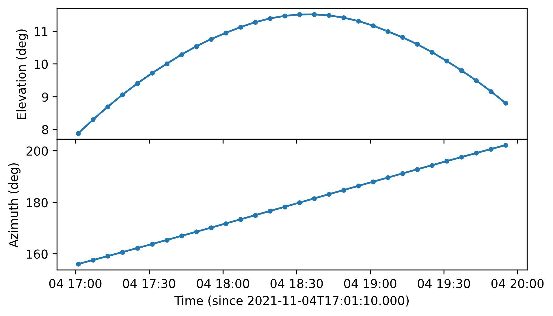
Analog pointing (horizontal coordinates) vs. time for a Jupiter observation.
Note
Another file is present in each NenuFAR observation repository: the so-called ‘tracking file’. This one lists the analog pointing orders used to control the delay lines. It looks like:
2021-11-04T17:01:10Z A 000 036 003 1 59 2 31
2021-11-04T17:01:10Z A 001 009 025 1 60 2 31
2021-11-04T17:01:10Z A 003 108 111 1 62 2 31
2021-11-04T17:01:10Z A 004 018 015 1 57 2 31
...
It is possible to reproduce these numbers, for checking purposes, using the MiniArray class.
For instance, the first line corresponds to the first time step, and the first Mini-Array (index 000).
We can read that the Xdelay and the Ydelay values are respectively 036 and 003.
From the .altazA file, above, we also read that the pointing order for the first time step, once the corrections are applied, is \((\phi=156.0355^{\circ}, \theta=7.8797^{\circ})\).
Using the hidden _skycoord_to_order() method, which takes as input a SkyCoord object for simplicity (that we set using the pointing coordinates), it is possible to find back these delay lines commands:
>>> from nenupy.instru import MiniArray
>>> from astropy.coordinates import SkyCoord
>>> import astropy.units as u
>>> ma = MiniArray(index=0)
>>> ma._skycoord_to_order(SkyCoord(156.0355, 7.8797, unit="deg"))
(36, 3)
altazB file
An .altazB file describes the numerical pointing of the NenuFAR array in beamforming operating mode.
Several numerical beams can co-exist (see NenuFAR pointing for more details), each with a given index BEAM.
Each numerical beam is linked to an analog beam (Mini-Arrays configuration), this is why the analog beam index ANA is associated to each line.
; ============================================================================================================
;YYYY-MM-DD HH:NN:SS  ANA BEAM  az (deg)   el (deg)           L                   M                   N
2021-11-04T17:01:10Z 0000 0000  155.3005   23.6678   0.382712881554200  -0.832095381992832   0.401432591550169
2021-11-04T17:01:20Z 0000 0000  155.3424   23.6800   0.382068139460654  -0.832297062149275   0.401628605986626
2021-11-04T17:01:30Z 0000 0000  155.3843   23.6923   0.381423336401039  -0.832498308203545   0.401824346309349
2021-11-04T17:01:40Z 0000 0000  155.4262   23.7045   0.380778195290465  -0.832699277533139   0.402019749747604
2021-11-04T17:01:50Z 0000 0000  155.4682   23.7167   0.380132857849189  -0.832899897616823   0.402214831816647
2021-11-04T17:02:00Z 0000 0000  155.5102   23.7289   0.379487324256145  -0.833100168358094   0.402409592592706
2021-11-04T17:02:10Z 0000 0000  155.5521   23.7411   0.378841591781727  -0.833300083263546   0.402604048128252
...
This file can directly be used to instantiate a Pointing.
The plot() method can be used to quickly visualize the pointings orders:
>>> altaz_b = ".../20211104_170000_20211104_200000_JUPITER_TRACKING.altazB"
>>> pointing = Pointing.from_file(file_name=altaz_b, beam_index=0)
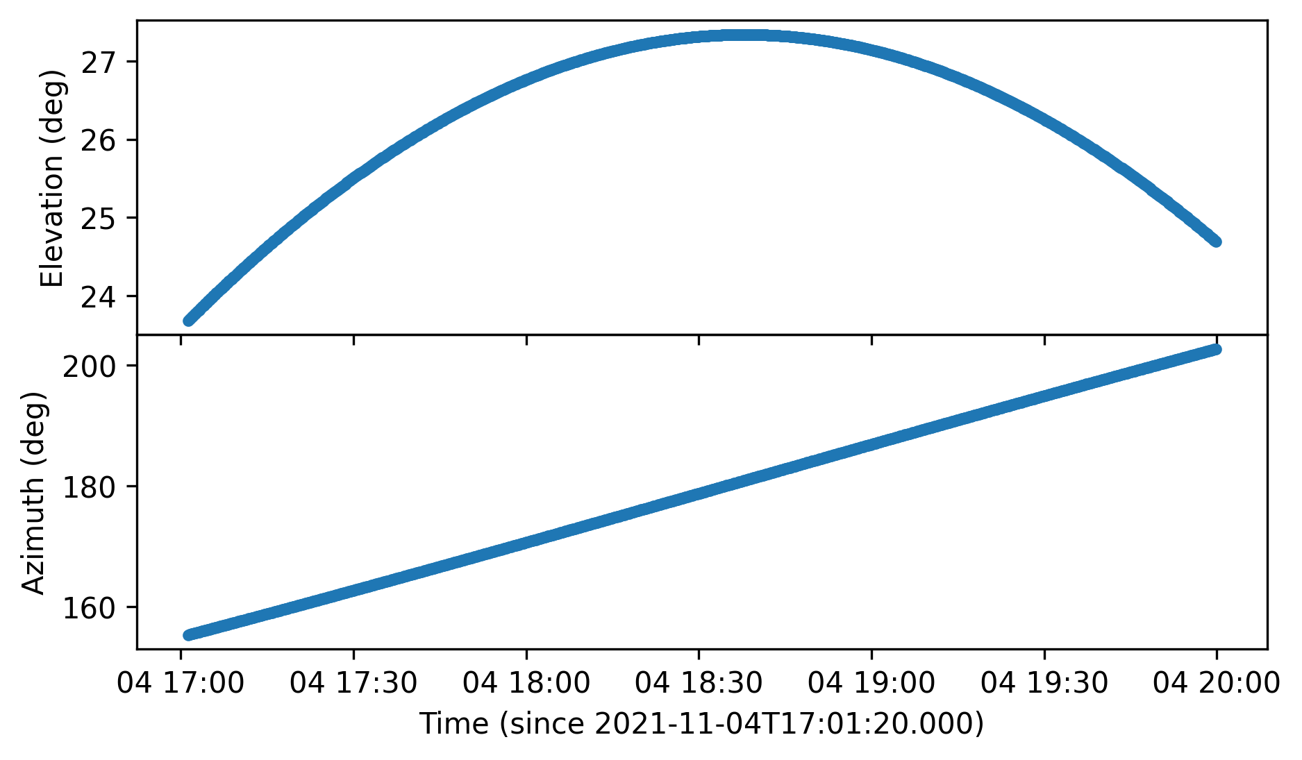
Numerical pointing (horizontal coordinates) vs. time for a Jupiter observation.
Comparing the two last plots (made for the same observation), the Beam squint correction applied to the analog beam can clearly be seen. The pointed elevations, for the latter, are lower than the ones pointed by the numerical beam.