Astronomical Targets
Astronomical targets are handled distinctively according to their apparent position in the sky.
Therefore, they are treated in Fixed sources and Solar System objects thanks to two object classes: FixedTarget and SolarSystemTarget respectively.
Both of these objects inherit from the abstract class Target.
Warning
FixedTarget and SolarSystemTarget are well suited to describe individual targets.
Dealing with multiple sky positions at once are better represented by Sky objects, see Sky representation.
For the purpose of this page examples, a few packages should be loaded first:
>>> from nenupy.astro.target import FixedTarget, SolarSystemTarget
>>> from astropy.time import Time, TimeDelta
>>> from astropy.coordinates import SkyCoord
>>> import astropy.units as u
>>> import numpy as np
>>> import matplotlib.pyplot as plt
Source types
Dealing with apparent source positions at NenuFAR site, as well as computing NenuFAR Beam Simulation within the nenupy framework is managed using Target objects.
Fixed sources
For sources that are fixed in the equatorial grid, an instance of FixedTarget can be created:
for an arbitrary position in the sky:
>>> source = FixedTarget(coordinates=SkyCoord(300, 45, unit="deg"))
>>> source.is_circumpolar
True
where
is_circumpolarcan quickly tells if a source is circumpolar as seen from Nançay location,for a known source using the classmethod
from_name()(with a name that could be resolved by Simbad):>>> cyg_a = FixedTarget.from_name("Cyg A") >>> cyg_a.coordinates <SkyCoord (ICRS): (ra, dec) in deg (299.86815191, 40.73391574)>
Horizontal coordinates are computed and accessed through the horizontal_coordinates attributes, providing that time as been properly filled.
In the example below, the variable times consists of a time range of 24 steps, separated by one hour, starting from 2021-01-01.
An FixedTarget instance is created at the position of Cygnus A, using this time range.
The source elevation with respect to time can then easily be displayed:
>>> times = Time("2021-01-01 00:00:00") + np.arange(24)*TimeDelta(3600, format="sec")
>>> cyg_a = FixedTarget.from_name("Cyg A", time=times)
>>> plt.plot(times.datetime, cyg_a.horizontal_coordinates.alt)
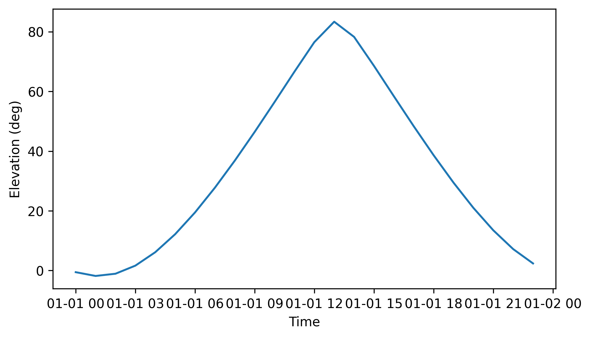
Cygnus A elevation vs. time as seen from NenuFAR on 2021-01-01.
Solar System objects
The Solar System planets and the Sun are not fixed in the equatorial grid and therefore require a distinct class able to handle the variations in sky positions over time.
The astropy.coordinates.solar_system_ephemeris are used to compute these positions.
An instance of SolarSystemTarget can be initialized with the classmethod from_name() for simplicity:
>>> times = Time("2021-01-01 00:00:00") + np.arange(24)*TimeDelta(3600, format="sec")
>>> sun = SolarSystemTarget.from_name("Sun", time=times)
>>> plt.plot(times.datetime, sun.horizontal_coordinates.alt)
As in Fixed sources, the Sun elevation is plotted against the time:
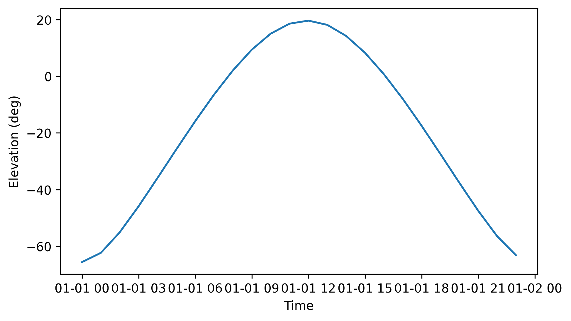
Sun elevation vs. time as seen from NenuFAR on 2021-01-01.
Knowing the apparent sky position of the Sun or any planet is straightforward:
>>> jupiter = SolarSystemTarget.from_name("Jupiter", time=Time("2021-11-18 16:00:00"))
>>> jupiter.horizontal_coordinates
<SkyCoord (AltAz: obstime=['2021-11-18 16:00:00.000'], location=(4323914.96644279, 165533.66845052, 4670321.74854012) m, pressure=0.0 hPa, temperature=0.0 deg_C, relative_humidity=0.0, obswl=1.0 micron): (az, alt) in deg
[(151.83875283, 23.68067178)]>
Ephemerides
Since both FixedTarget and SolarSystemTarget classes are sub-classes of Target, objects of these types are granted access to a range of methods bringing additional information on their ephemerides.
Namely, these are:
|
Computes the |
|
Computes the |
|
Computes the |
|
Computes the |
|
Computes the |
|
Computes the |
|
Computes the |
|
Computes the |
|
Computes the |
|
Computes the |
Meridian transit
Knowing the time of the meridian crossing is useful because it gives an indication on when the source is at its highest position in the sky (i.e., well suited for observations: NenuFAR antennas greatest sensitivity, low atmospheric effects, and the human activities not in the field of view).
meridian_transit() is the method to call for.
The meridian transit time is computed iteratively on smaller and smaller time windows, until the required precision is reached.
The example below illustrates how to compute the Sun meridian transit time occuring within a time slot ranging from t_min to t_min + duration:
>>> sun = SolarSystemTarget.from_name("Sun")
>>> sun.meridian_transit(
        t_min=Time("2021-11-04 00:00:00"),
        duration=TimeDelta(86400, format="sec")
    )
<Time object: scale='utc' format='iso' value=['2021-11-04 11:34:46.659']>
Note
The output of meridian_transit() is a Time array because there can possibly be several transit times between t_min and t_min + duration.
Two related methods (next_meridian_transit() and previous_meridian_transit()) are used to know the previous or next meridian transit time with respect to time:
>>> sun = SolarSystemTarget.from_name("Sun")
>>> sun.next_meridian_transit(time=Time("2021-11-04 00:00:00"))

<Time object: scale='utc' format='iso' value=2021-11-04 11:34:46.770>
>>> sun = SolarSystemTarget.from_name("Sun")
>>> sun.previous_meridian_transit(time=Time("2021-11-04 00:00:00"))

<Time object: scale='utc' format='iso' value=2021-11-03 11:34:45.664>
Azimuth transit
Sometimes, the computation of the transit time at a specific azimuth (other than the meridian plan) is required.
The method azimuth_transit() allows the user to give as input any azimuth value (as Quantity objects):
>>> sun = SolarSystemTarget.from_name("Sun")
>>> sun.azimuth_transit(
        t_min=Time("2021-11-04 00:00:00"),
        duration=TimeDelta(86400, format="sec"),
        azimuth=200*u.deg
    )

<Time object: scale='utc' format='iso' value=['2021-11-04 12:49:54.389']>
If the source does not cross the required azimuth between t_min and t_min + duration, then an empty object is returned:
>>> sun = SolarSystemTarget.from_name("Sun")
>>> sun.azimuth_transit(
        t_min=Time("2021-11-04 00:00:00"),
        duration=TimeDelta(86400, format="sec"),
        azimuth=10*u.deg
    )

<Time object: scale='utc' format='jd' value=[]>
Note
All the methods previously mentionned (meridian_transit(), next_meridian_transit(), previous_meridian_transit(), azimuth_transit())
can be tweaked with a precision argument, which reflects the smallest time window used while searching for transit times.
By default, this argument is set to 5 seconds, but this can be modified and the results may vary accordingly:
example with 1 minute precision:
>>> sun = SolarSystemTarget.from_name("Sun")
>>> sun.next_meridian_transit(
        time=Time("2021-11-04 00:00:00"),
        precision=TimeDelta(60, format="sec")
    )

<Time object: scale='utc' format='iso' value=2021-11-04 11:34:03.418>
example with 1 second precision:
>>> sun = SolarSystemTarget.from_name("Sun")
>>> sun.next_meridian_transit(
        time=Time("2021-11-04 00:00:00"),
        precision=TimeDelta(1, format="sec")
    )

<Time object: scale='utc' format='iso' value=2021-11-04 11:34:47.477>
Multiple transits
meridian_transit() and azimuth_transit() (as well as rise_time() and set_time(), see Rise and set times) will return as many ouptuts as there are occurences within the time window looked upon (i.e., between t_min and t_min + duration).
Therefore, searching for the Sun meridian transit times over two days returns a Time array of two elements:
>>> sun = SolarSystemTarget.from_name("Sun")
>>> two_days = TimeDelta(48*3600, format="sec")
>>> sun.meridian_transit(t_min=Time("2021-11-04 00:00:00"), duration=two_days)

<Time object: scale='utc' format='iso' value=['2021-11-04 11:34:46.770' '2021-11-05 11:34:47.876']>
In the example below, a time range over a three-day period is created and stored in the variable times.
The radio source Cygnus A is instantiated (as an FixedTarget object), while setting its time attribute to times.
The meridian transit times are computed using meridian_transit() and stored in transits.
Finally, a plot is made to show Cygnus A elevation while highlighting the transit times just found:
>>> # Define the time range
>>> time_steps = 72
>>> three_days = TimeDelta(72*3600, format="sec")
>>> times = Time("2021-01-01 00:00:00") + np.arange(time_steps)*three_days/time_steps

>>> # Compute the meridian transit times
>>> cyg_a = FixedTarget.from_name("Cyg A", time=times)
>>> transits = cyg_a.meridian_transit(t_min=times[0], duration=three_days)

>>> # Plot the elevation vs. time, and the transit times as vertical lines
>>> plt.plot( times.datetime, cyg_a.horizontal_coordinates.alt)
>>> for transit in transits:
>>>     plt.axvline(transit.datetime, color="black")
>>> plt.xlabel("Time")
>>> plt.ylabel("Elevation (deg)")
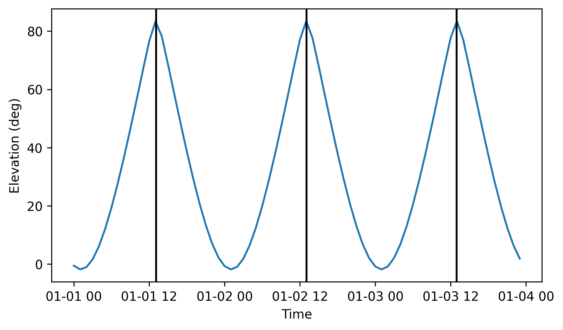
Cygnus A elevation vs. time (blue curve). The meridian transit times are displayed as vertical black lines.
Rise and set times
Computing rise and set times of a Target instance is done in a similar fashion.
Below, the methods rise_time() and set_time() are used to compute the rise and set time of Cygnus A above and below an elevation of 20 deg.
>>> # Define the time range
>>> time_steps = 72
>>> three_days = TimeDelta(72*3600, format="sec")
>>> times = Time("2021-01-01 00:00:00") + np.arange(time_steps)*three_days/time_steps

>>> # Compute the rise and set times where the elevation crosses 20 deg
>>> cyg_a = FixedTarget.from_name("Cyg A", time=times)
>>> rises = cyg_a.rise_time(times[0], elevation=20*u.deg, duration=three_days)
>>> sets = cyg_a.set_time(times[0], elevation=20*u.deg, duration=three_days)

>>> # Plot the elevation vs. time, and the crossing times as vertical lines
>>> plt.plot(times.datetime, cyg_a.horizontal_coordinates.alt)
>>> for r in rises:
>>>     plt.axvline(r.datetime, color="black", linestyle='-.')
>>> for s in sets:
>>>     plt.axvline(s.datetime, color="black", linestyle=':')
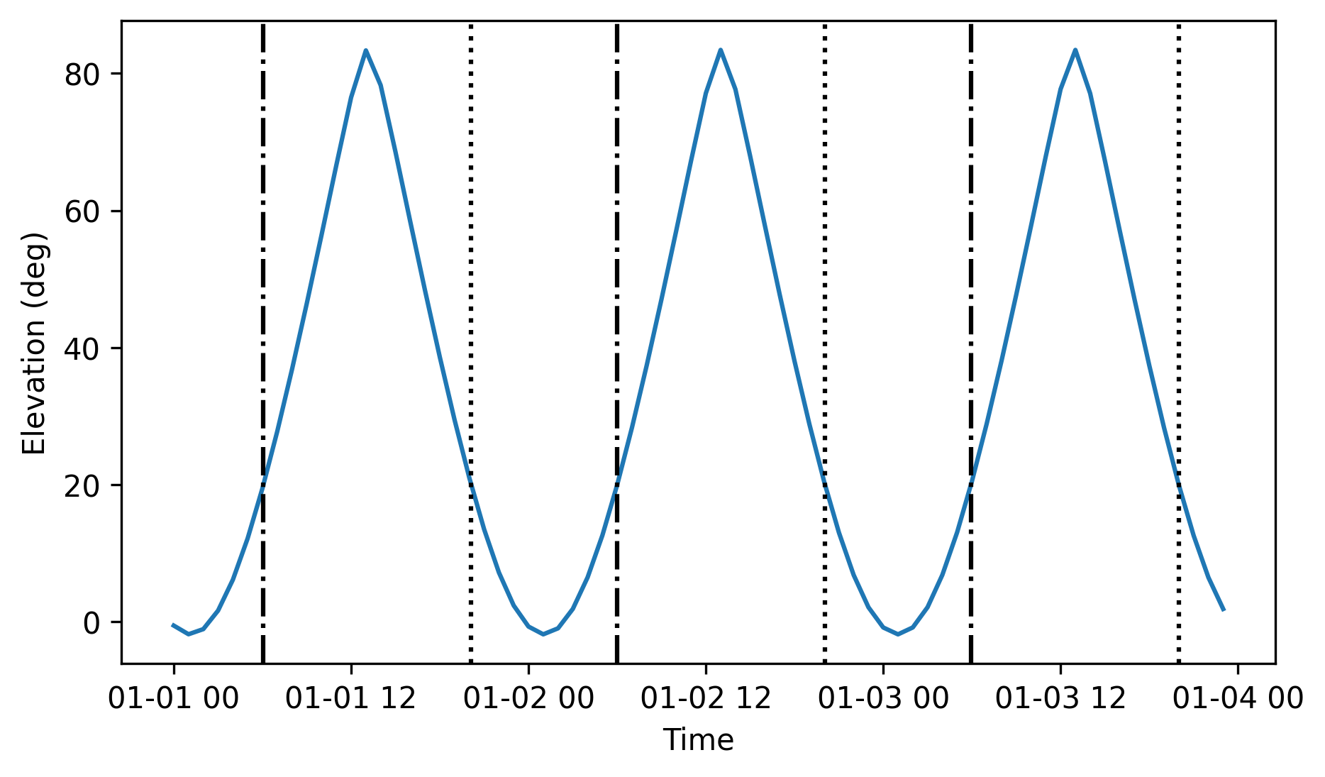
Cygnus A elevation vs. time (blue curve). The rise times when the source goes above an elevation of 20 deg are highlighted as dashed-dotted vertical black lines. The set times when the source goes below an elevation of 20 deg are highlighted as dotted vertical black lines.