Beamforming from XST

Cross-correlation statistics data (or XST), although mainly used in the NenuFAR ‘proto-imager’ mode and for the NenuFAR-TV (see XST Imaging tutorial), can be suited to achieve different purposes. Indeed, they contain recorded amplitude and phase data for each baseline involved in the observation. Hence their ability to be converted to beamformed statistics data (or BST) at will. This can in particular be done for any subset of Mini-Arrays in any pointing direction allowing for numerous potential array configurations available at once with a single XST observation, rather than performing as many BST observations as desired configurations.

The following tutorial aims at reproducing an existing BST observation (here a Cygnus A meridian transit observed with different East-West orientated Mini-Array pairs: '20191129_141900_BST.fits') with the corresponding XST data taken at the same time ('20191129_141900_XST.fits').

Both data sets are loaded using BST_Data and XST_Data classes and stored as bst and xst instances respectively:

>>> from nenupy.beamlet import BST_Data
>>> from nenupy.crosslet import XST_Data
>>> bst = BST_Data('20191129_141900_BST.fits')
>>> xst = XST_Data('20191129_141900_XST.fits')

The BST data contains four array configurations corresponding to four pairs of different Mini-Arrays. Selection of the first configuration is done by setting dbeam index to 0. The selected configurations involves the pair of Mini-Arrays 16 and 51 (checked with mas attribute). The final comparison will be on a single frequency time profile indexed freq_idx. BST data are selected accordingly with the select() method and giving freqrange the XST frequency corresponding to freq_idx index:

>>> freq_idx = 1
>>> bst.dbeam = 0
>>> bst_d = bst.select(
        freqrange=xst.freqs[freq_idx]
    )

Beamforming the cross-correlation data is done using beamform() method. The phasing direction must be given in local sky coordinates. Hence, to compare the BST and XST data, the pointing direction (azdig and eldig) stored in the BST file metadata are given to az (azimuth) and el (elevation) parameters. The ma parameter is set with the selected Mini-Array pair (mas), although it could accept any subset of Mini-Arrays. The polarization pol is such as the current selected BST polarization: polar. Finally, the calibration table is specified ('default' value enables the calibration table used during the BST observation). bst_d and xst_d are both SData objects.

>>> xst_d = xst.beamform(
        az=bst.azdig[0],
        el=bst.eldig[0],
        pol=bst.polar,
        ma=bst.mas,
        calibration='default'
    )

Warning

XST beamforming in tracking mode is not enabled yet.

Corresponding BST observation can be simulated using from_bst() method (see Observation simulations tutorial for more details):

>>> from nenupy.simulation import HpxSimu
>>> from astropy.time import TimeDelta
>>> simu = HpxSimu.from_bst(
        bst,
        dt=TimeDelta(60, format='sec'),
        resolution=0.5
    )

simu is another SData object, and everything can de displayed together for comparison:

>>> import matplotlib.pyplot as plt
>>> plt.plot(
        xst_d.datetime,
        xst_d.db[:, freq_idx],
        label='{} from XST'.format(bst.polar),
        linewidth=8
    )
>>> plt.plot(
        bst_d.datetime,
        bst_d.db,
        label='{} from BST'.format(bst.polar),
        linewidth=1.5
    )
>>> scale = np.median(bst_d.db) / np.median(simu.db)
>>> plt.plot(
        simu.datetime,
        simu.db * scale,
        label='{} from BST simulation'.format(bst.polar)
    )
>>> plt.legend()
>>> plt.ylabel('dB')
>>> plt.xlabel('Time since {}'.format(bst.time[0].isot))
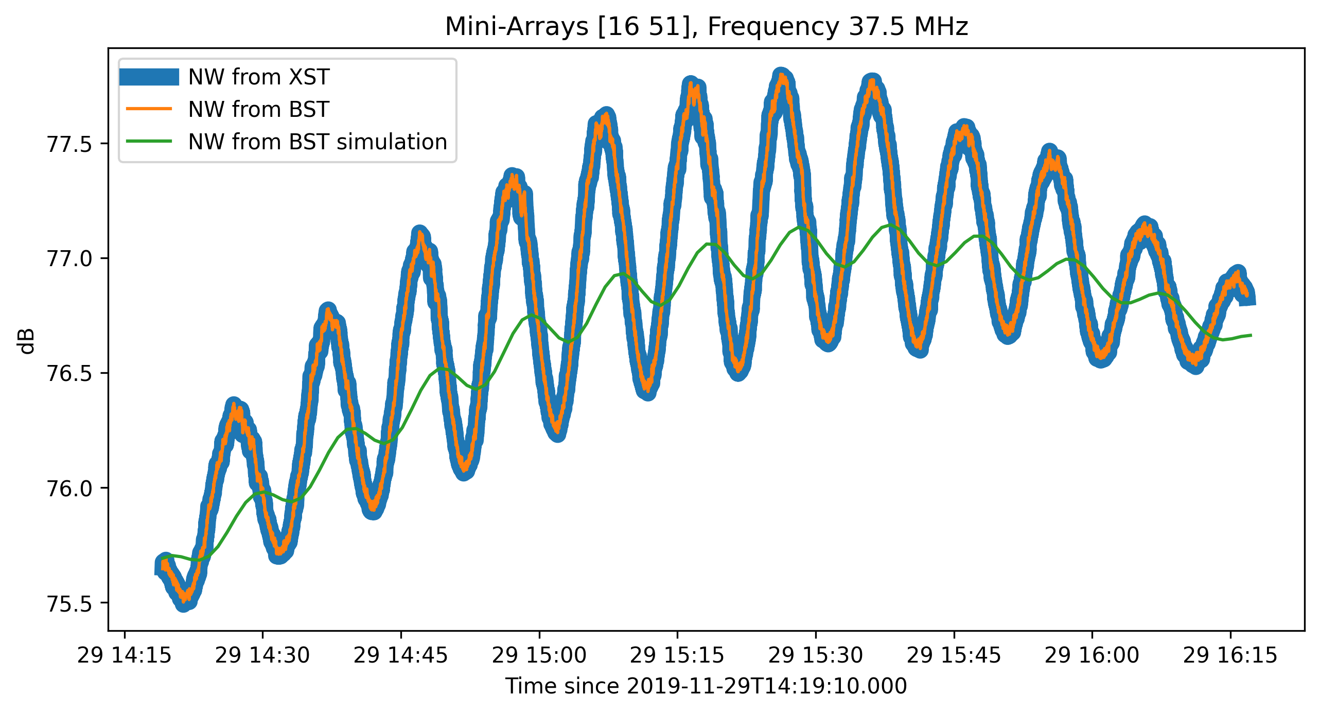
>>> plt.title('Mini-Arrays {}, Frequency {}'.format(bst.mas, xst.freqs[freq_idx]))

Note

The above figure shows in blue the time-profile at 37.5 MHz obtained from beamforming the XST observation and in orange the corresponding BST profile. Both are perfectly identical, as expected. The Mini-Array pair being roughly East-West orientated implies North-South beam fringes. The meridian transit of Cygnus A thus appears like a sinusoidal curve. The corresponding simulation is shown in green and some discrepancies can be noted: lower fringe amplitudes (mostly due to Cygnus A not being a perfect point source in the GSM skymodel) and phase-shift of the fringes (maybe due to a slight instrument shift from ideal pointing).

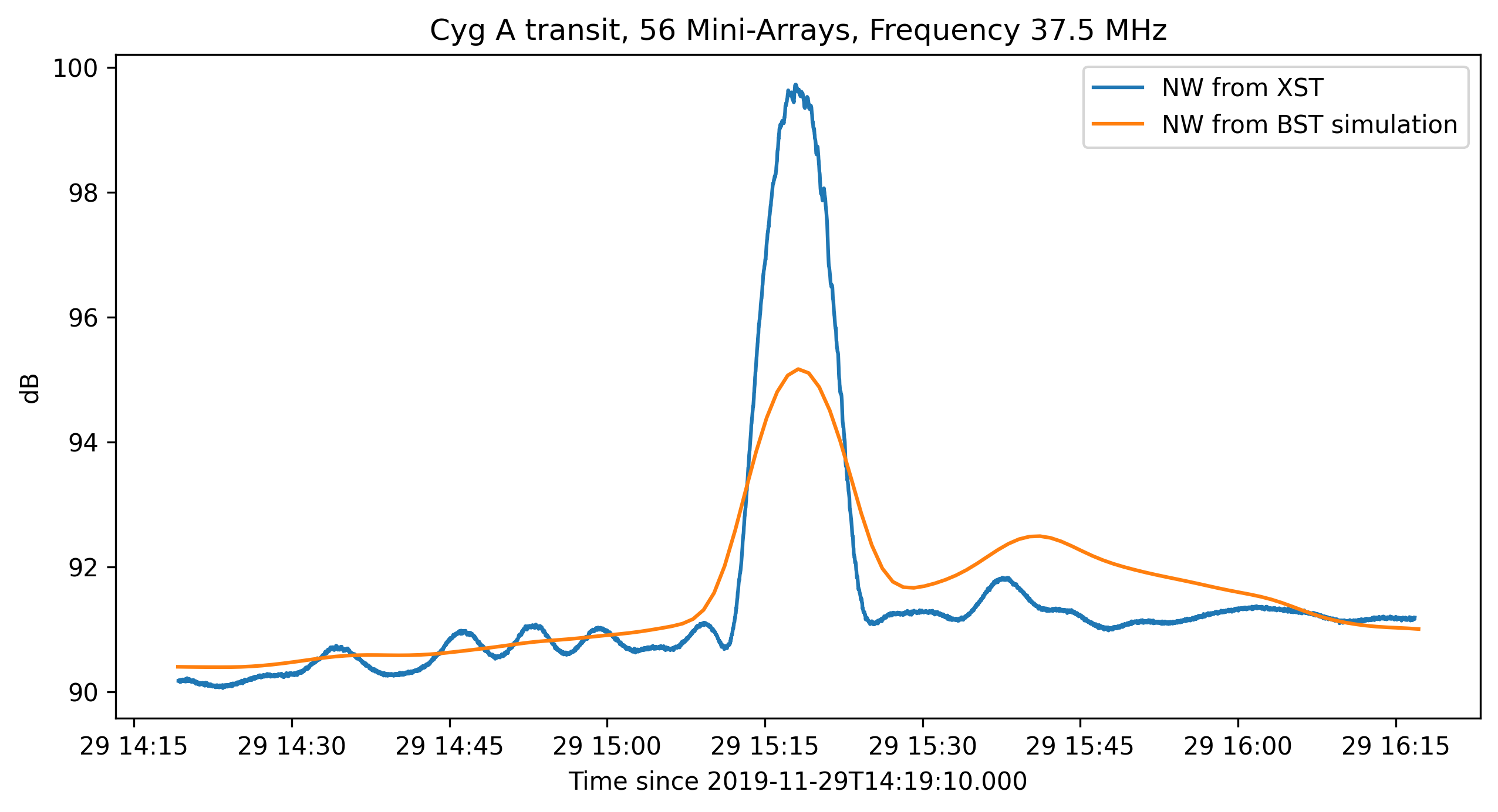
The same dataset can also be used to beamform any subset of NenuFAR Mini-Arrays, in particular the whole array. miniarrays variable is a list of the 56 Mini-Arrays names:

>>> miniarrays = np.arange(56)

The beamform() method is once again called with this new Mini-Array subset in input, and the results are stored in the SData object bst_d:

>>> bst_d = xst.beamform(
        az=bst.azdig[0],
        el=bst.eldig[0],
        pol=bst.polar,
        ma=miniarrays,
        calibration='default'
    )

A simulation can also be made using the (almost) same array configuration while calling azel_transit() after having defined a coordinate object with ho_coord():

>>> from nenupy.astro import ho_coord
>>> transit_altaz = ho_coord(
        az=bst.azdig[0],
        alt=bst.eldig[0],
        time=bst.times[0]
    )
>>> simu = HpxSimu(
        freq=xst.freqs[freq_idx],
        resolution=0.5,
        ma=miniarrays,
        polar=bst.polar
    )
>>> exposure = bst.times[-1] - bst.times[0]
>>> result = simu.azel_transit(
        acoord=transit_altaz,
        t0=bst.times[0] + exposure/2.,
        dt=TimeDelta(60, format='sec'),
        duration=exposure,
    )

Note

It should be noted that the reconstructed beamformed observation (blue curve) was made with only 8 Mini-Arrays analog phased towards the meridian transit of Cygnus A, the other 48 were default phased at the local zenith. However, the simulation (orange curve) assumed that the 56 Mini-Arrays were analog phased towards the target. This, in addition to the skymodel uncertainties, are the main caveats for this comparison interpretation.