NenuFAR Beam Simulation

NenuFAR instrument simulations represent a core feature of nenupy. They are used for the commissioning work, for the Observation Simulations (in data quality assesment and features identification), and also for skymodel preparation (as input for imaging calibration). This page describes the Beam simulation principle to learn the main mandatory steps and the general philosophy of beam simulation. Then, in the following are detailed hierarchically the methods to simulate the Antenna radiation pattern, the Mini-Array response, and the NenuFAR array beam.

Several nenupy modules are rquired in order to perform beam simulation:

>>> from nenupy.instru import MiniArray, NenuFAR, Polarization, NenuFAR_Configuration
>>> from nenupy.astro.sky import HpxSky
>>> from nenupy.astro.pointing import Pointing
>>> from nenupy.astro.target import FixedTarget, SolarSystemTarget

And below are few other generic packages that are useful to load:

>>> from astropy.time import Time, TimeDelta
>>> import astropy.units as u
>>> import numpy as np

Beam simulation quickstart

It is sometimes useful to quickly check the state of the beam during an observation. Beam simulations could help identifying whether a particular feature in the data could come from bright sources. Prior to observing, the check is also relevant as it could assess the correct observation configuration. The function plot_current_pointing() takes in input the analog pointing file (ending by “.altazA”) automatically generated at every observation by the NenuFAR systems (can be found in the Virtual Control Room or in nancep servers under /databf/nenufar). It simulates the analog beam (i.e., comprised of the 6 various Mini-Array rotations) at the selected time and frequency, taking into account realistic pointing orders:

>>> from nenupy.observation import plot_current_pointing
>>> import astropy.units as u
>>> from astropy.time import Time

>>> plot_current_pointing(
        figname="my_beam_simulation.png",
        time=Time("2026-03-12 12:00:00"),
        frequency=50 * u.MHz,
        analog_pointing_file="20260312_101200_20260312_135000_SUN_TRACKING.altazA",
        source_positions=True,
        contour_values=False
    )

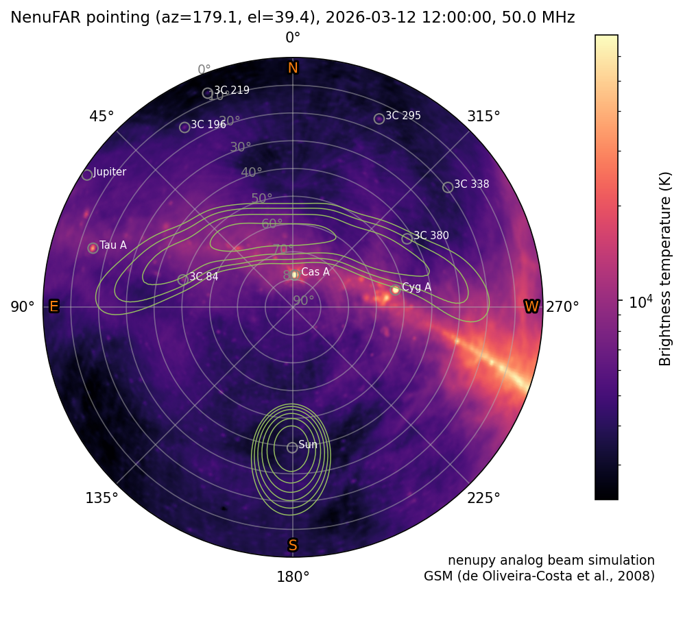
NenuFAR analog beam simulation during a Solar observation, projected in an azimuth-elevation polar frame. Contours are defined on a logarithmic scale to better enhance the grating ring, that is partially viewed in this example. The radio sky is displayed in the background to identify bright source positions and Galactic plane orientation with respect to the beam.

Beam simulation principle

The beam simulation involves a few steps:

• An instrument array should be created (of type Interferometer), which, in the NenuFAR case, means instantiation of either MiniArray or NenuFAR. The array element can be configured as desired (see Array Configuration for more details):

  >>> instrument = NenuFAR()
  

• Instrumental Pointing should be described (see Instrument Pointing for more details and pointing options):

  >>> simulation_dt = TimeDelta(1800, format="sec")
  >>> simulation_times = Time("2021-01-01 12:00:00") + np.arange(12)*simulation_dt
  >>> zenith = Pointing.zenith_tracking(
          time=simulation_times,
          duration=simulation_dt
      )
  

• Then, the requested simulation output should be precised, as a Sky (or HpxSky) instance (see Sky representation). The simulation will then be performed for each time, frequency, polarization and coordinates:

  >>> whole_sky = HpxSky(
          resolution=0.5*u.deg,
          frequency=np.array([25, 50, 75])*u.MHz,
          polarization=Polarization.NW,
          time=simulation_times
      )
  

• Finally, the simulation is made using nenupy.instru.nenufar.MiniArray.beam() or nenupy.instru.nenufar.NenuFAR.beam() (with sky and pointing arguments filled with inputs previously defined). Note that the bulk of the computation is not yet performed, for the simulation (stored in the value attribute) is a dask.array.Array object:

  >>> simulated_beam = instrument.beam(sky=whole_sky, pointing=zenith)
  

• The results are stored in the simulated_beam variable in this example which is of the same type as whole_sky. The shape is (time, frequency, polarization, coordinates):

  >>> simulated_beam.value
          Array               Chunk
  Bytes   54.00 MiB               4.50 MiB
  Shape   (12, 3, 1, 196608)      (1, 3, 1, 196608)
  Count   192 Tasks               12 Chunks
  Type    float64             numpy.ndarray
  

Antenna radiation pattern

The NenuFAR antenna radiation pattern depends on the selected polarization (defined while instantiating Sky). There are two available polarization values, defined as within the enum class Polarization: NW and NE.

In the example below, the antenna variable is created from instantiating MiniArray with only one antenna. The antenna_response is computed using beam(). A plot() is made from a slice on the HpxSky object ([8, 0, 0] means 9th time steps, first frequency value, first polarization value). Whenever an operation is performed on such selection, the computation is run:

>>> antenna = MiniArray()["Ant10"]
>>> antenna_response = antenna.beam(sky=whole_sky, pointing=zenith)
>>> antenna_response[8, 0, 0].plot(altaz_overlay=True)

Note

The zenithal pointing has no effect here since the individual NenuFAR antenna are not steerable.

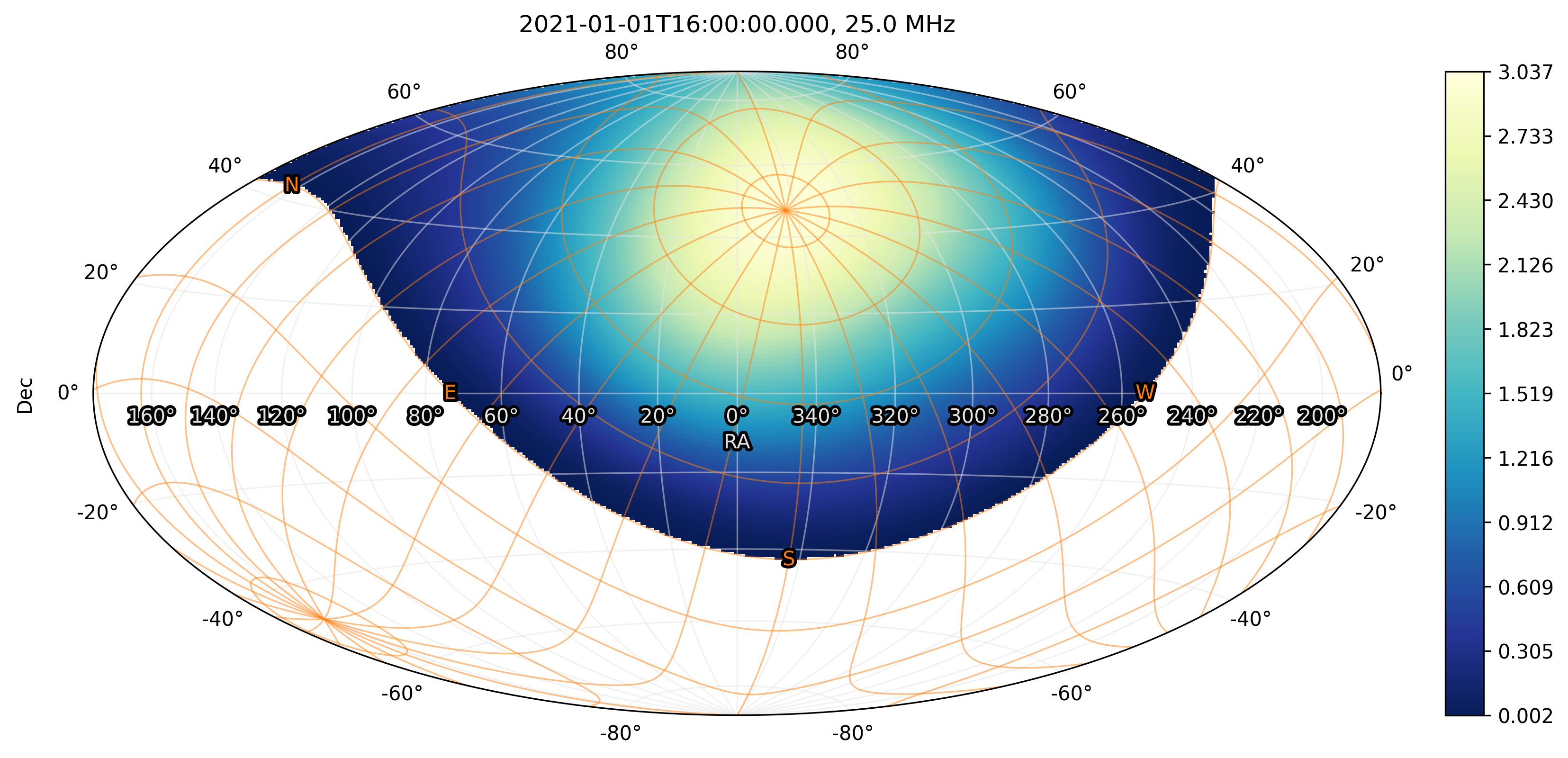
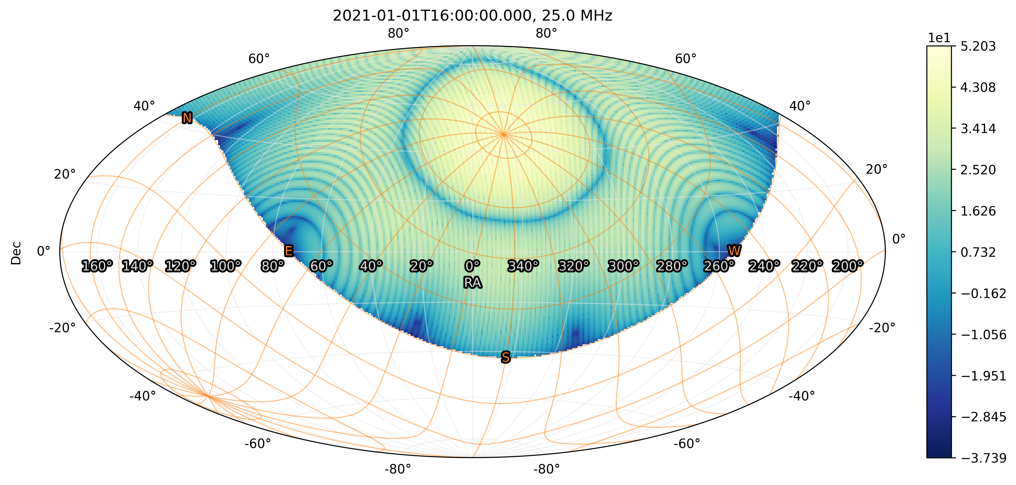
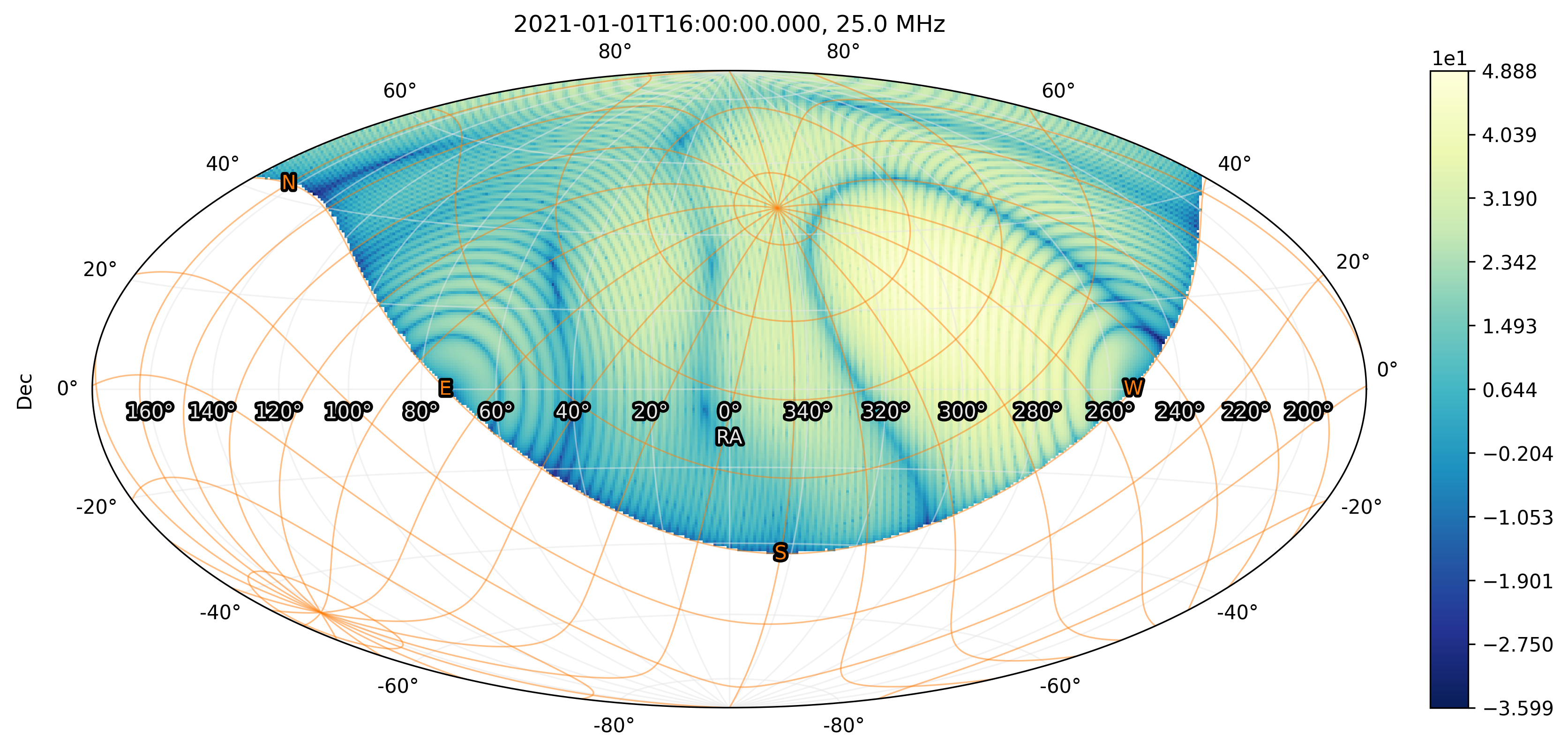
NenuFAR antenna radiation pattern, polarization NW, 25 MHz, as seen from Nançay. Only the sky above the horizon is represented. The horizontal coordinates are displayed as an orange grid.

Mini-Array response

The NenuFAR Mini-Array response can be computed in the same way. After instantiating MiniArray, the beam() method is called. This time, the plot() from a different slice, where the third frequency index is selected (corresponding to 75 MHz):

>>> ma = MiniArray()
>>> beam = ma.beam(sky=whole_sky, pointing=zenith)
>>> beam[8, 2, 0].plot(altaz_overlay=True)

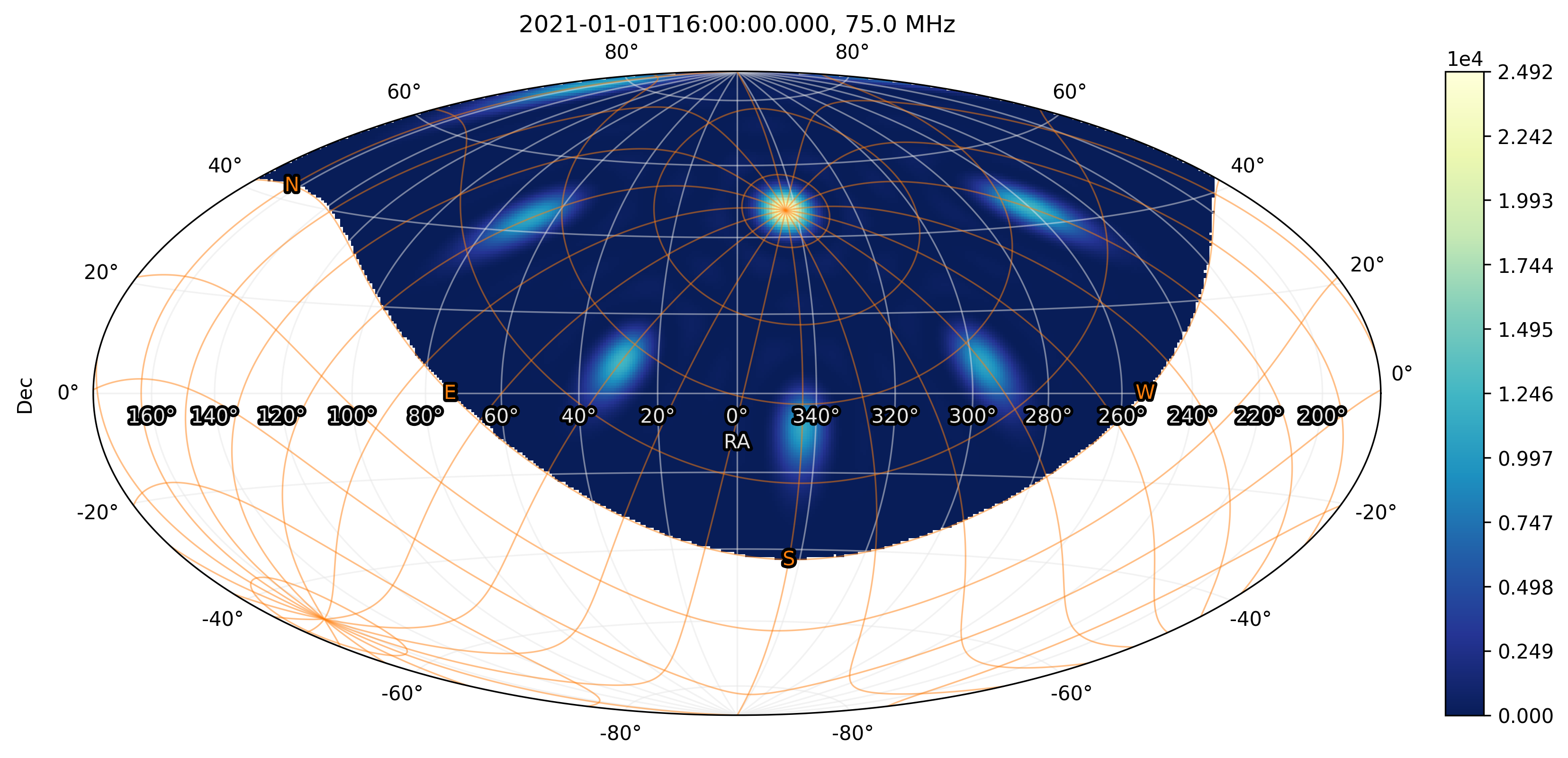
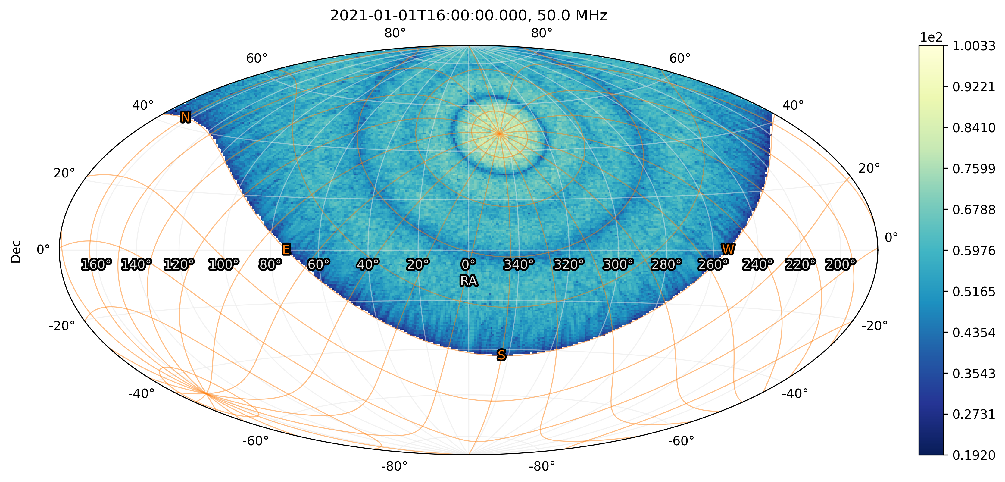
NenuFAR Mini-Array radiation pattern, polarization NW, 75 MHz, as seen from Nançay. Only the sky above the horizon is represented. The horizontal coordinates are displayed as an orange grid.

Beam squint correction

Radio phased array are affected by beam squint. The combination between the antenna response (maximal at zenith) and the array factor of an antenna distribution can shift the maximal sensitivity towards greater elevations. To correct this effect, the Mini-Array pointing elevation is shifted a little bit lower than desired (this is done by the method beamsquint_correction()).

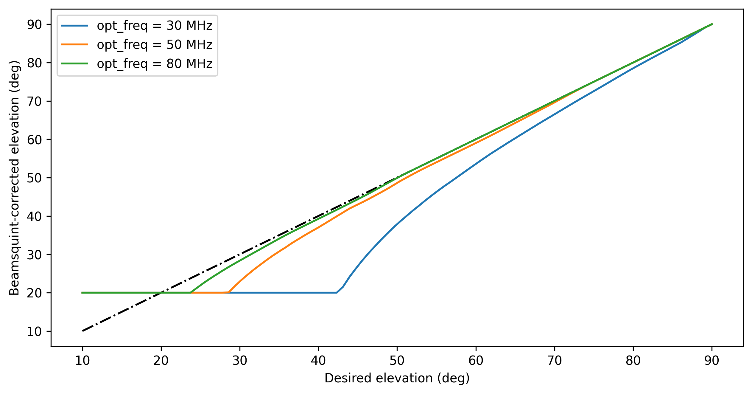
Beamsquint-corrected elevation vs. desired elevation. The correction is frequency-dependent and is greater at low elevation.

To visualize this effect, a tracking on a given source position is set. And the simulation is performed over the entire sky (whole_sky).

>>> source = SkyCoord(320, 10, unit="deg")
>>> source_tracking = Pointing.target_tracking(
        target=FixedTarget(coordinates=source),
        time=Time("2021-01-01 18:00:00")
    )
>>> whole_sky = HpxSky(
        resolution=0.5*u.deg,
        frequency=25*u.MHz,
        polarization=Polarization.NW,
        time=Time("2021-01-01 18:00:00")
    )
>>> ma = MiniArray()

The beamsquint correction is first deactivated thanks to NenuFAR_Configuration. The following figure shows that the Mini-Array beam maximal sensitivity is located at a higher elevation with respect to the source position.

>>> conf = NenuFAR_Configuration(
        beamsquint_correction=False,
    )
>>> beam = ma.beam(sky=whole_sky, pointing=source_tracking, configuration=conf)
>>> beam[0, 0, 0].plot(
        altaz_overlay=True,
        scatter=(source, 50, "tab:red"),
        contour=(beam[0,0,0].value.compute(), None, "copper")
    )

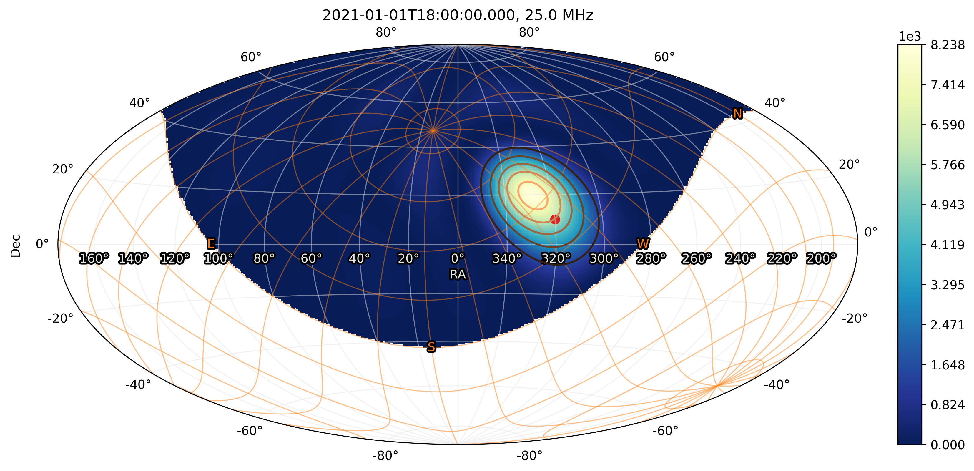
Mini-Array beam simulation at 25 MHz. The beamsquint correction is deactivated. The source position is marked as a red dot. Horizontal coordinates are represented as an orange grid.

For comparison, the beamsquint correction is activated (default mode). The correction frequency beamsquint_frequency is set to match the observing frequency.

>>> conf = NenuFAR_Configuration(
        beamsquint_correction=True,
        beamsquint_frequency=30*u.MHz
    )
>>> beam = ma.beam(sky=whole_sky, pointing=source_tracking, configuration=conf)
>>> beam[0, 0, 0].plot(
        altaz_overlay=True,
        scatter=(source, 50, "tab:red"),
        contour=(beam[0,0,0].value.compute(), None, "copper")
    )

With the correction in place, the Mini-Array beam peaks closer to the apparent source position.

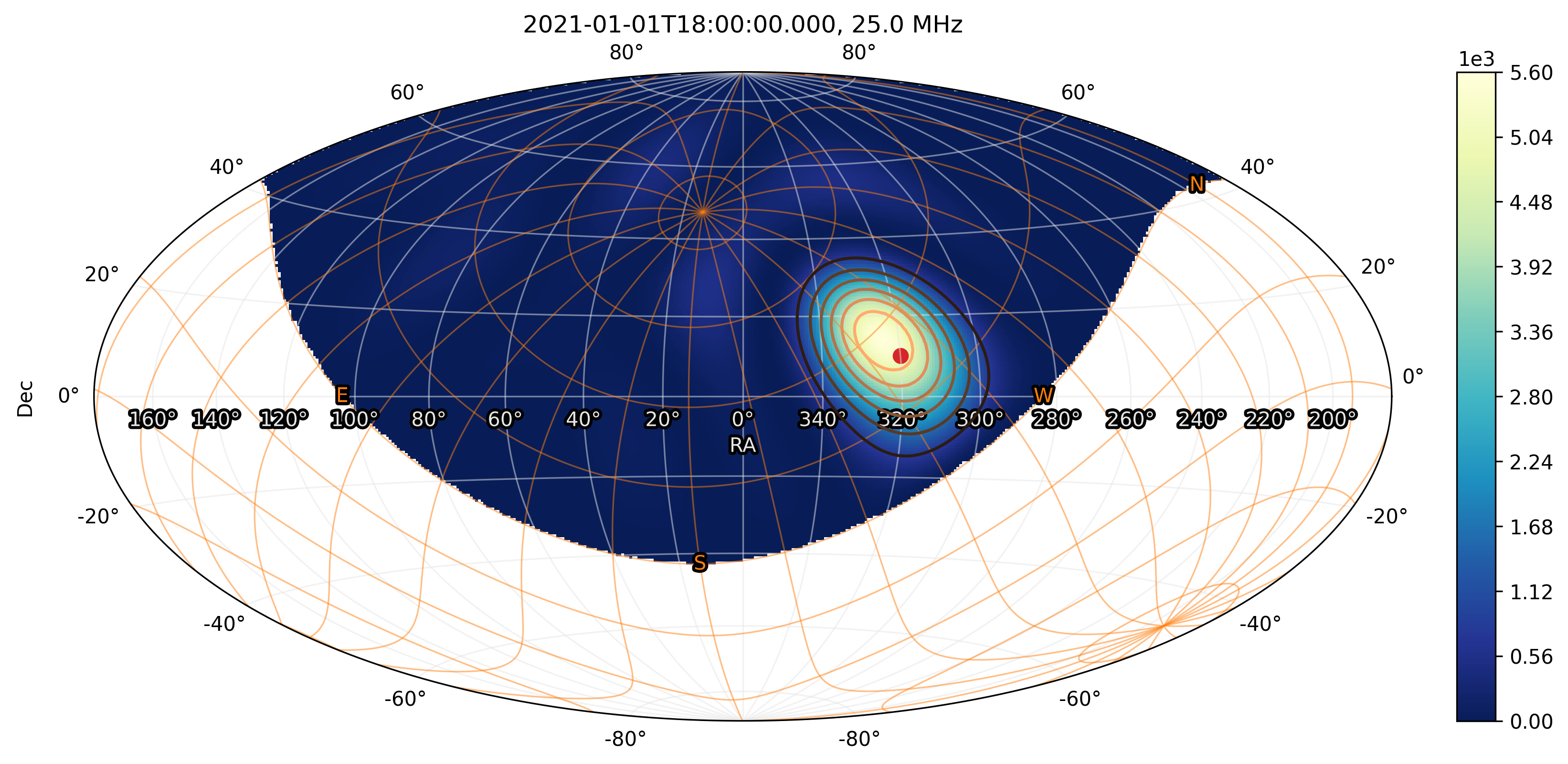
Mini-Array beam simulation at 25 MHz. The beamsquint correction is activated. The source position is marked as a red dot. Horizontal coordinates are represented as an orange grid.

Discrete beam simulation

All the above examples have been run with a HpxSky sky as input. That is, using a HEALPix representation of the entire sky (see HEALPix sky representation). Sometimes, however, a reduced number of and/or more specifics coordinates are needed.

The class Sky is an alternative, where the user can set the desired coordinates for which the beam simulation should be performed. This is particularly true for sky model alteration during the imaging calibration process.

>>> from astropy.coordinates import SkyCoord
>>> # Observation times
>>> dt = TimeDelta(1800, format="sec")
>>> obs_times = Time("2021-01-01 12:00:00") + np.arange(12)*dt
>>> # North Celestial Pole tracking
>>> ncp = FixedTarget.from_name("North Celestial Pole")
>>> ncp_tracking = Pointing.target_tracking(
        target=ncp,
        time=obs_times,
        duration=dt
    )
>>> # Discrete sky grid
>>> ra, dec = np.meshgrid(
        np.linspace(0, 360, 100),
        np.linspace(-90, 90, 100)
    )
>>> sky = Sky(
        coordinates=SkyCoord(ra, dec, unit="deg").ravel(), # it needs to be 1D
        time=obs_times,
        frequency=70*u.MHz,
        polarization=Polarization.NW
    )
>>> # Array definition
>>> ma = MiniArray()
>>> # Beam simulation and plotting
>>> beam = ma.beam(sky=sky, pointing=ncp_tracking)
>>> beam[0, 0, 0].plot()

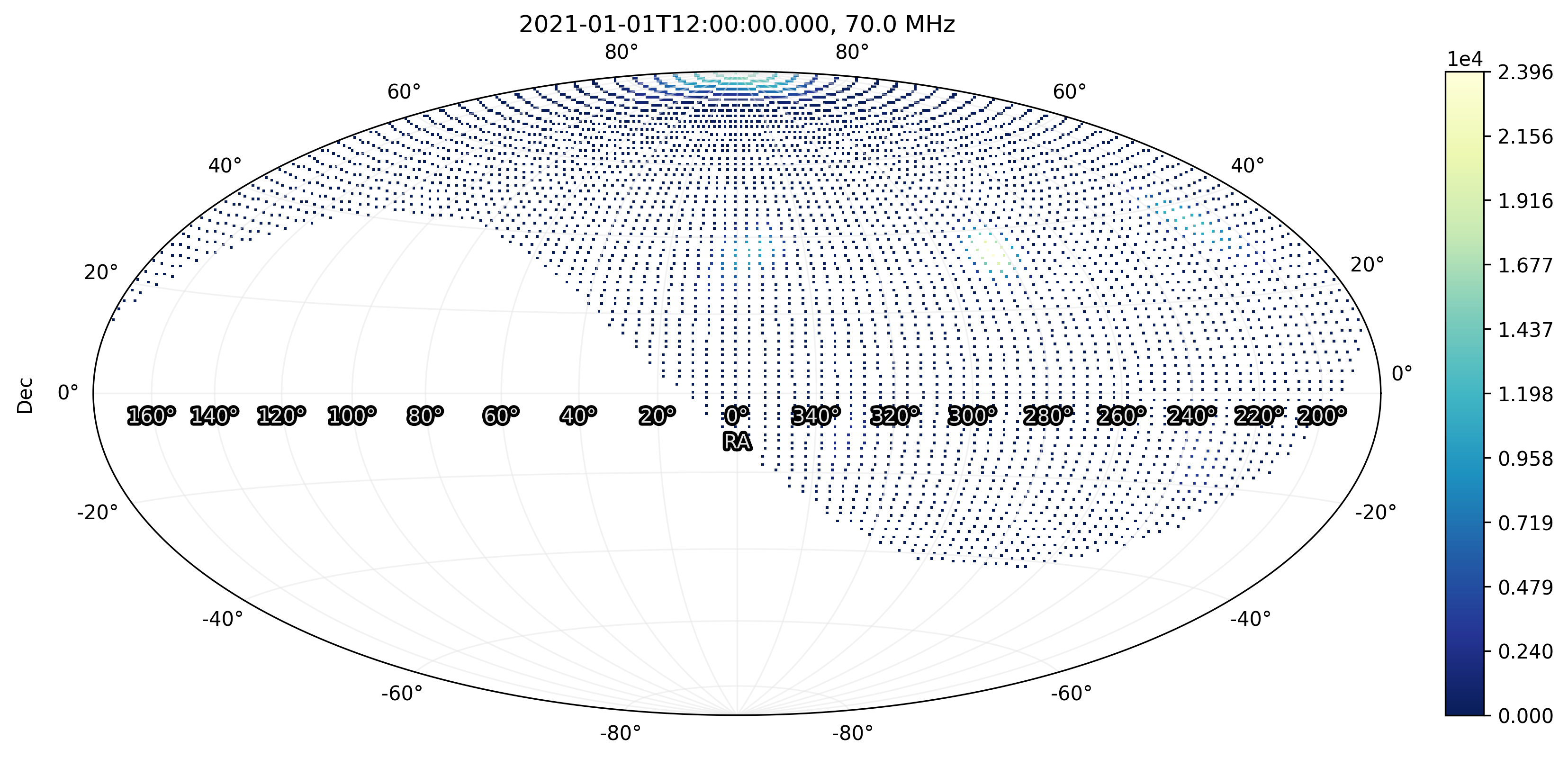
Mini-Array beam simulation of a North Celestial Pole tracking made on a grid of custom sky positions.

NenuFAR array beam

Finally, beam simulation of the NenuFAR array can be performed, providing that a NenuFAR instance is created. The method beam() is used.

Sub-set of NenuFAR array

Any NenuFAR configuration is accepted. For instance, the following example details the beam simulation of NenuFAR consisting of only two Mini-Arrays (namely 040 et 055). These two Mini-Arrays are roughly located on an East-West axis, implying that the array factor should display North-South stripes (see the figure below).

>>> nenufar = NenuFAR()["MA040", "MA055"]
>>> beam = nenufar.beam(sky=whole_sky, pointing=zenith)
>>> beam[8, 0, 0].plot(altaz_overlay=True, decibel=True)

Beam simulation of NenuFAR with only two Mini-Arrays.

Often during NenuFAR beamforming observations, the analog pointing is different from the numerical one. It is therefore possible to give another Pointing object to the beam() method via its argument analog_pointing. Below, an arbitrary pointing other_pointing, away from the numerical pointing (which produces the North-South stripes), is given. The Mini-Array response is then different than the one above.

>>> other_pointing = Pointing.target_tracking(
        target=FixedTarget(coordinates=SkyCoord(300, 20, unit="deg")),
        time=simulation_times,
        duration=simulation_dt
    )
>>> nenufar = NenuFAR()["MA040", "MA055"]
>>> beam = nenufar.beam(
        sky=whole_sky,
        pointing=zenith,
        analog_pointing=other_pointing
    )
>>> beam[8, 0, 0].plot(altaz_overlay=True, decibel=True)

Beam simulation of NenuFAR with only two Mini-Arrays. An arbitrary pointing towards \((\alpha=300^{\circ}, \delta=20^{\circ}\) has been set for the anaog pointing.

Whole NenuFAR core response

The 96 core Mini-Array response can be computed in a straightforward manner:

>>> nenufar = NenuFAR()
>>> beam = nenufar.beam(sky=whole_sky, pointing=zenith)
>>> beam[8, 1, 0].plot(altaz_overlay=True, decibel=True)

Zenith beam simulation with 96 Mini-Arrays at 50 MHz.

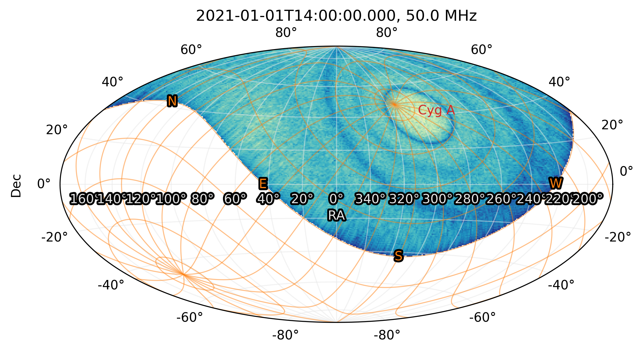
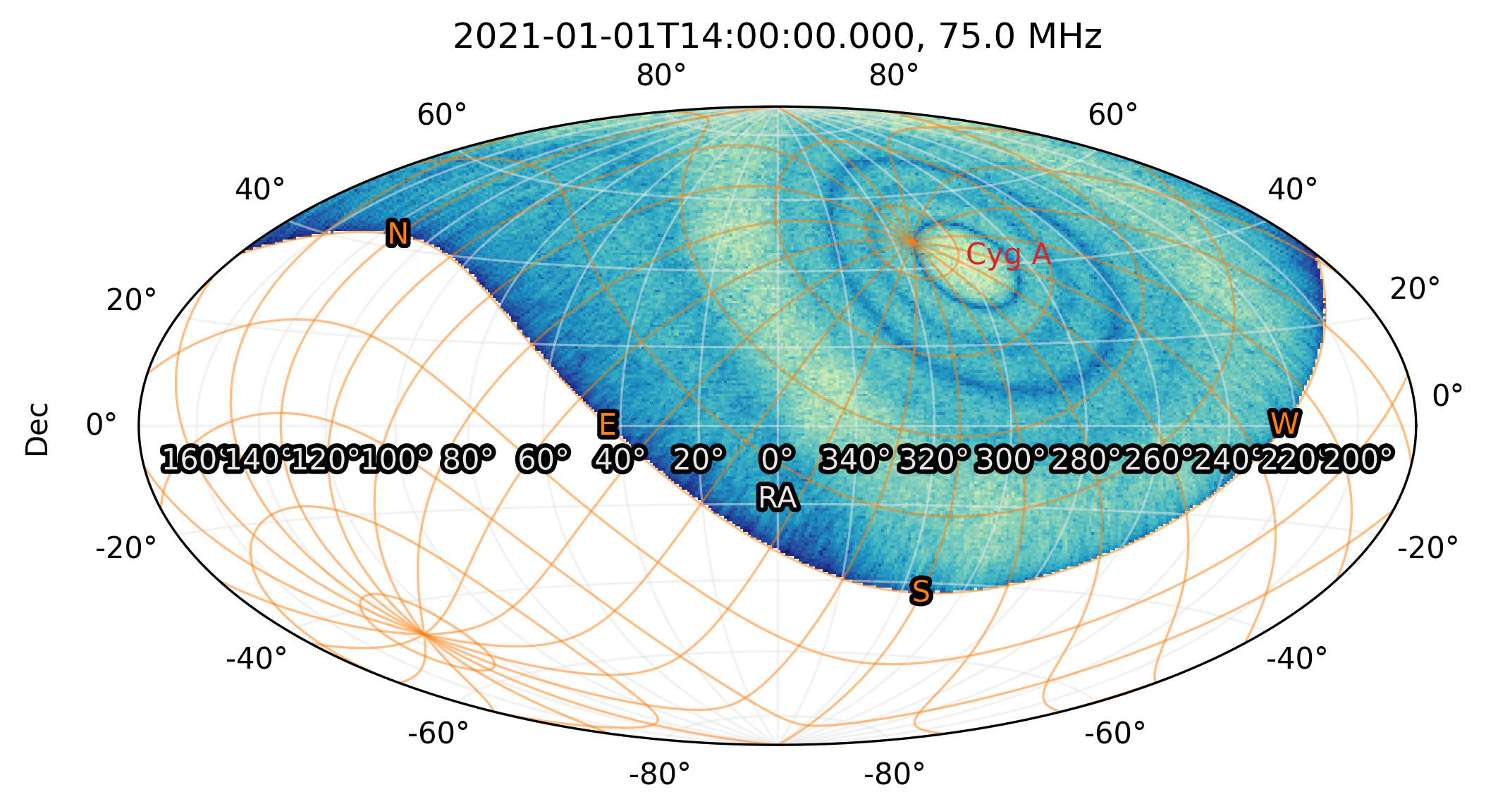
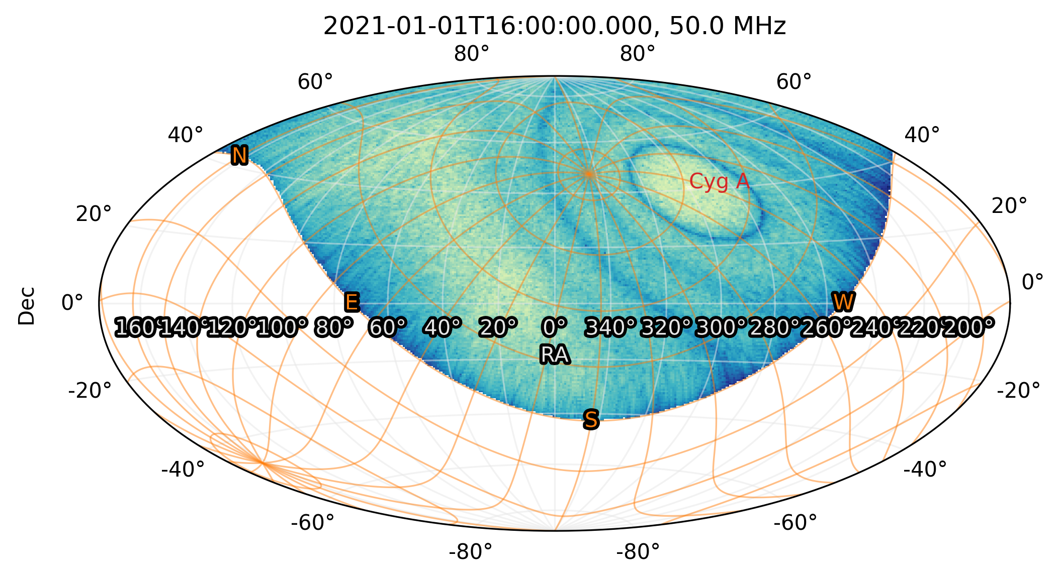
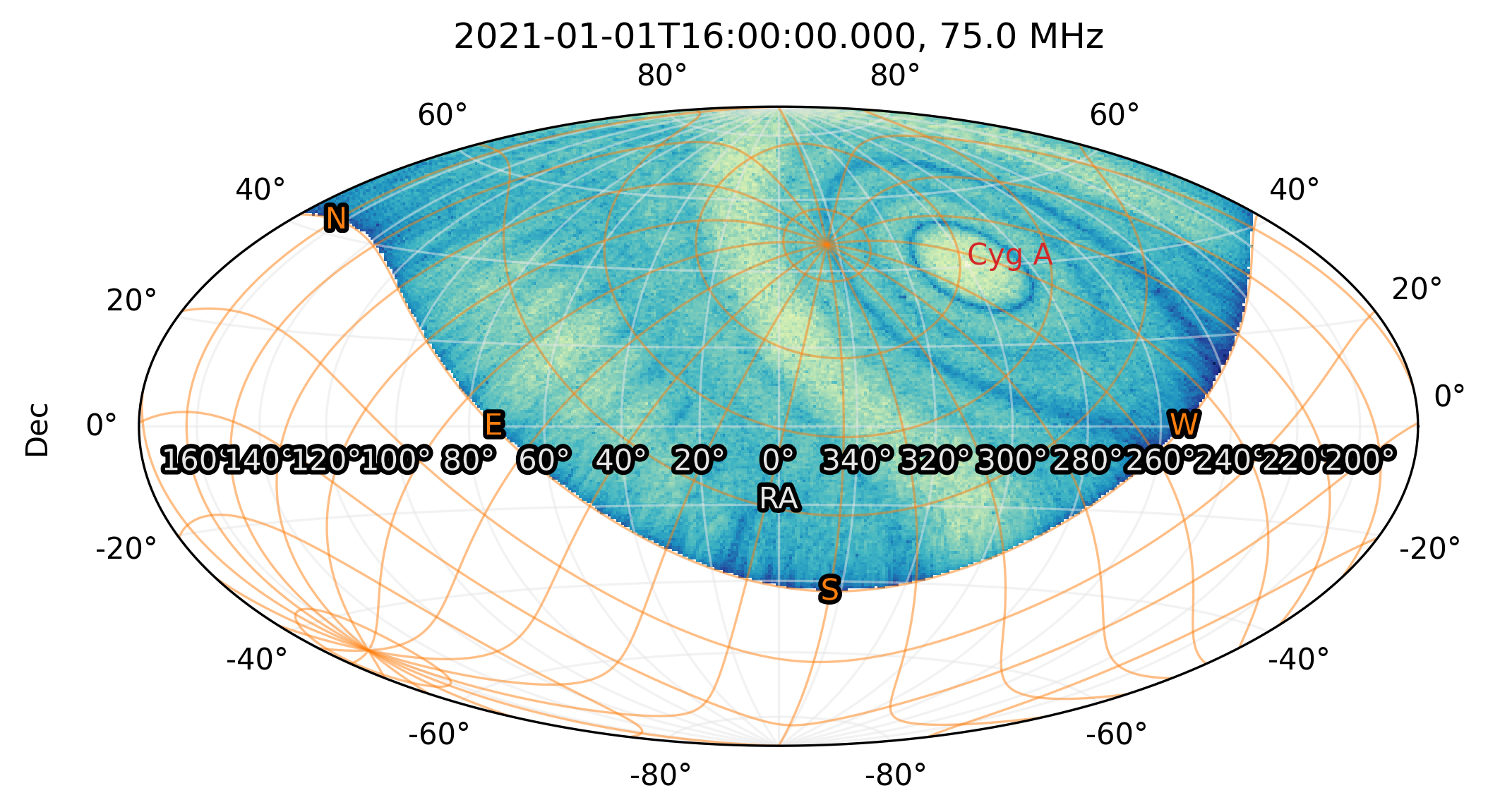
Example (tracking Cygnus A)

This last example brings everything that has been discussed previousy together and aims at understanding the slicing of the output simulation. A simulation of the whole NenuFAR core array is performed over 3 time steps, 2 frequency values and 1 polarization.

>>> # 3 time steps, separated by 2 hours
>>> dt = TimeDelta(7200, format="sec")
>>> times = Time("2021-01-01 12:00:00") + np.arange(3)*dt
>>> # Cygnus A tracking
>>> cyga = FixedTarget.from_name("Cygnus A")
>>> cyga_tracking = Pointing.target_tracking(
        target=cyga,
        time=times,
        duration=dt
    )
>>> # HEALPix sky definition at two frequencies, one polarization
>>> whole_sky = HpxSky(
        resolution=0.5*u.deg,
        frequency=np.array([50, 75])*u.MHz,
        polarization=Polarization.NW,
        time=times
    )
>>> # Instantiation of the full NenuFAR core array
>>> nenufar = NenuFAR()
>>> # Beam simulation
>>> beam = nenufar.beam(sky=whole_sky, pointing=cyga_tracking)

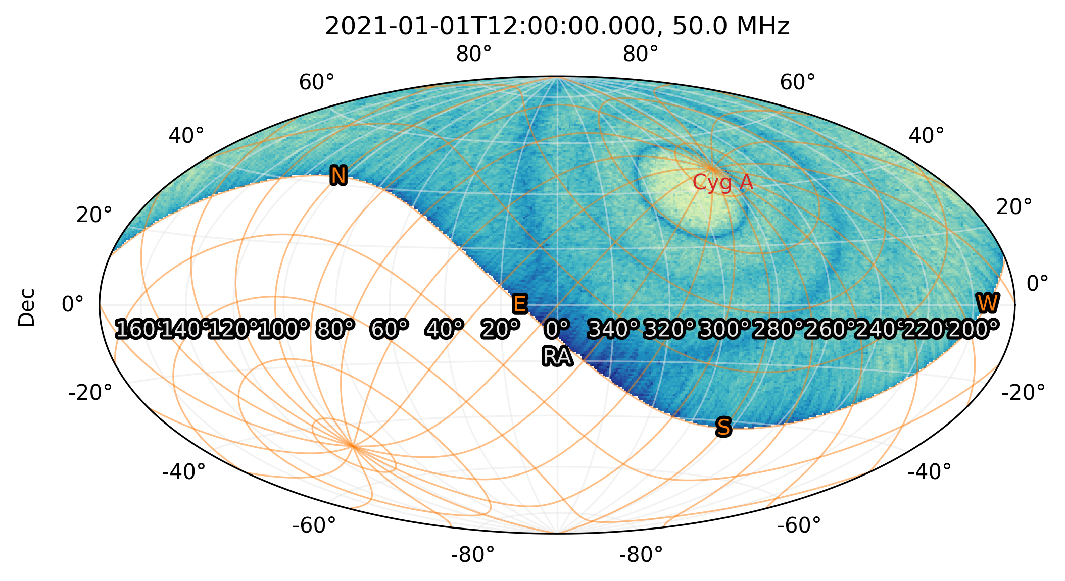
Slicing the beam object as [time, frequency, polarization] gives access to the various time and frequency values contained in the simulation:

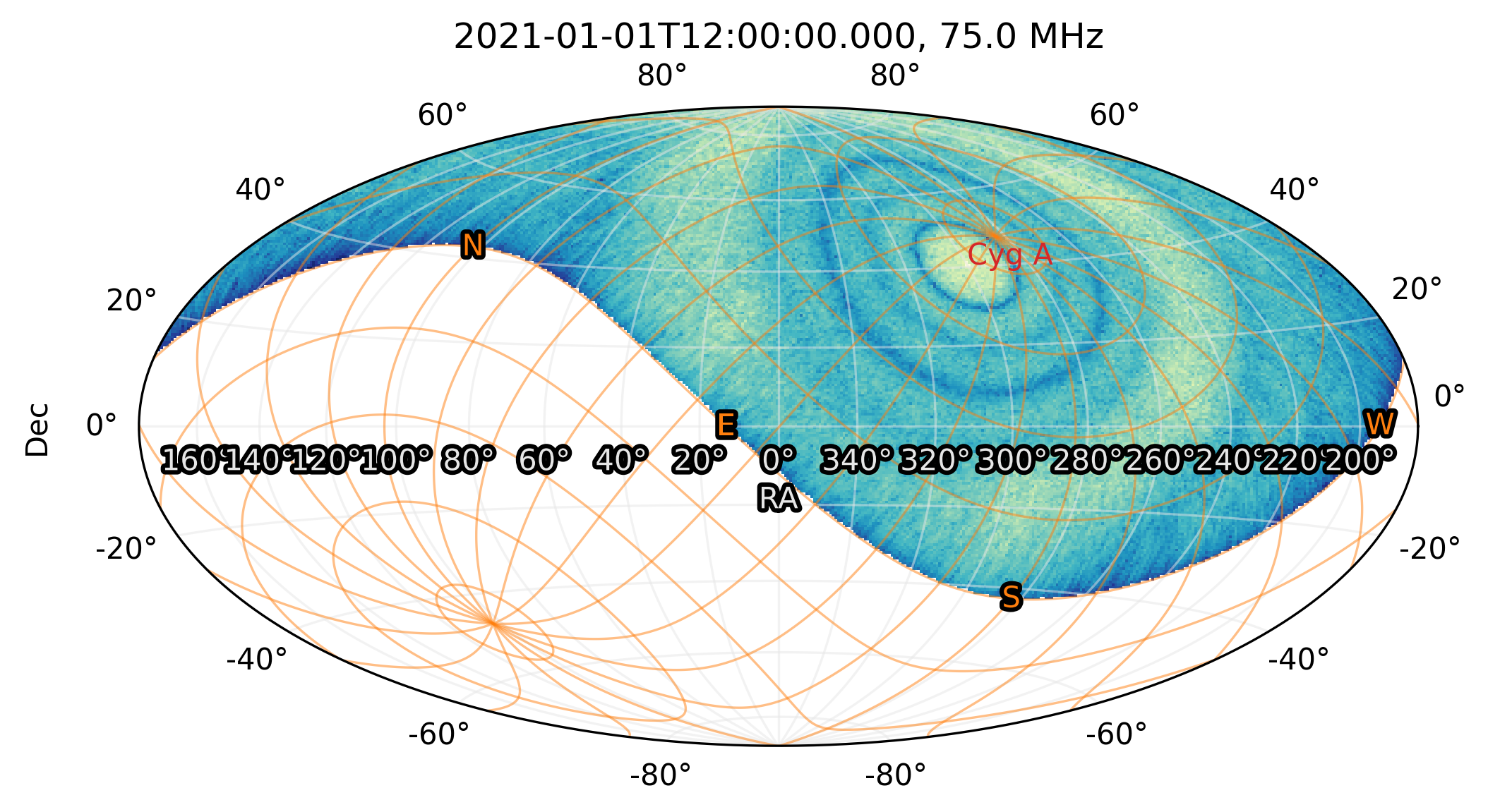
>>> beam[0, 0, 0].plot(decibel=True)	>>> beam[0, 1, 0].plot(decibel=True)
>>> beam[1, 0, 0].plot(decibel=True)	>>> beam[1, 1, 0].plot(decibel=True)
>>> beam[2, 0, 0].plot(decibel=True)	>>> beam[2, 1, 0].plot(decibel=True)