Cross-Correlation STatistics (XST)

NenuFAR produces cross-correlation statistics data called XST that can be converted to Measurement Set format suited for radio imaging softwares (this is the ‘proto-imager’ mode, in contrast with the proper imager mode using data from the NICKEL correlator).

When NenuFAR does not observe in XST mode, the cross-correlations are saved with 10 sec integration time and 16 sub-bands of 195.3125 kHz in 5-min exposure time binary files. They are immediately converted in images to be displayed as the NenuFAR-TV and near-field images are also produced.

NenuFAR Cross-Correlation Statistics come in two flavours, namely XST FITS files and NenuFAR-TV binary files. They can be read and analyzed by XST and NenufarTV respectively. Both classes inherit from the base class Crosslet, which contains the methods to extract, and perform basic imaging and beamforming operations.

XST selection

Reading a NenuFAR XST file is straightforward with XST. The general information may be displayed using info(), and some specific file type dependent properties may be accessed by dedicated attributes, such as mini_arrays:

>>> from nenupy.io.xst import XST

>>> xst = XST(".../nenupy/tests/test_data/XST.fits")
>>> xst.info()
file: '.../nenupy/tests/test_data/XST.fits'
frequency (1, 16): 68.5546875 MHz -- 79.296875 MHz
time (1,): 2020-02-19T18:00:03.000 -- 2020-02-19T18:00:03.000
data: (1, 16, 6105)

>>> xst.mini_arrays
array([ 0,  2,  3,  4,  5,  6,  7,  8,  9, 10, 11, 12, 13, 14, 15, 16, 17,
   18, 19, 20, 21, 22, 23, 24, 25, 26, 27, 28, 29, 30, 31, 32, 33, 34,
   35, 36, 37, 38, 39, 40, 41, 42, 43, 44, 45, 46, 47, 48, 49, 50, 51,
   52, 53, 54, 55], dtype='>i2')

Data selection can then be applied either using get() or get_stokes() methods. The former accesses the raw cross-correlations stored in the FITS files (namely the polarizations “XX”, “XY”, “YX” and “YY”), the latter adds a Stokes parameter computation layer.

>>> from nenupy.io.xst import XST

>>> xst = XST(".../nenupy/tests/test_data/XST.fits")
>>> xx_data = xst.get(
        polarization="XX",
        miniarray_selection=None,
        frequency_selection=">=20MHz",
        time_selection=">=2020-02-19T18:00:00"
    )

Both methods return an instance of the class XST_Slice which contains the methods to further process the data, as well as plotting tools such as plot_correlaton_matrix():

>>> xx_data.plot_correlaton_matrix()

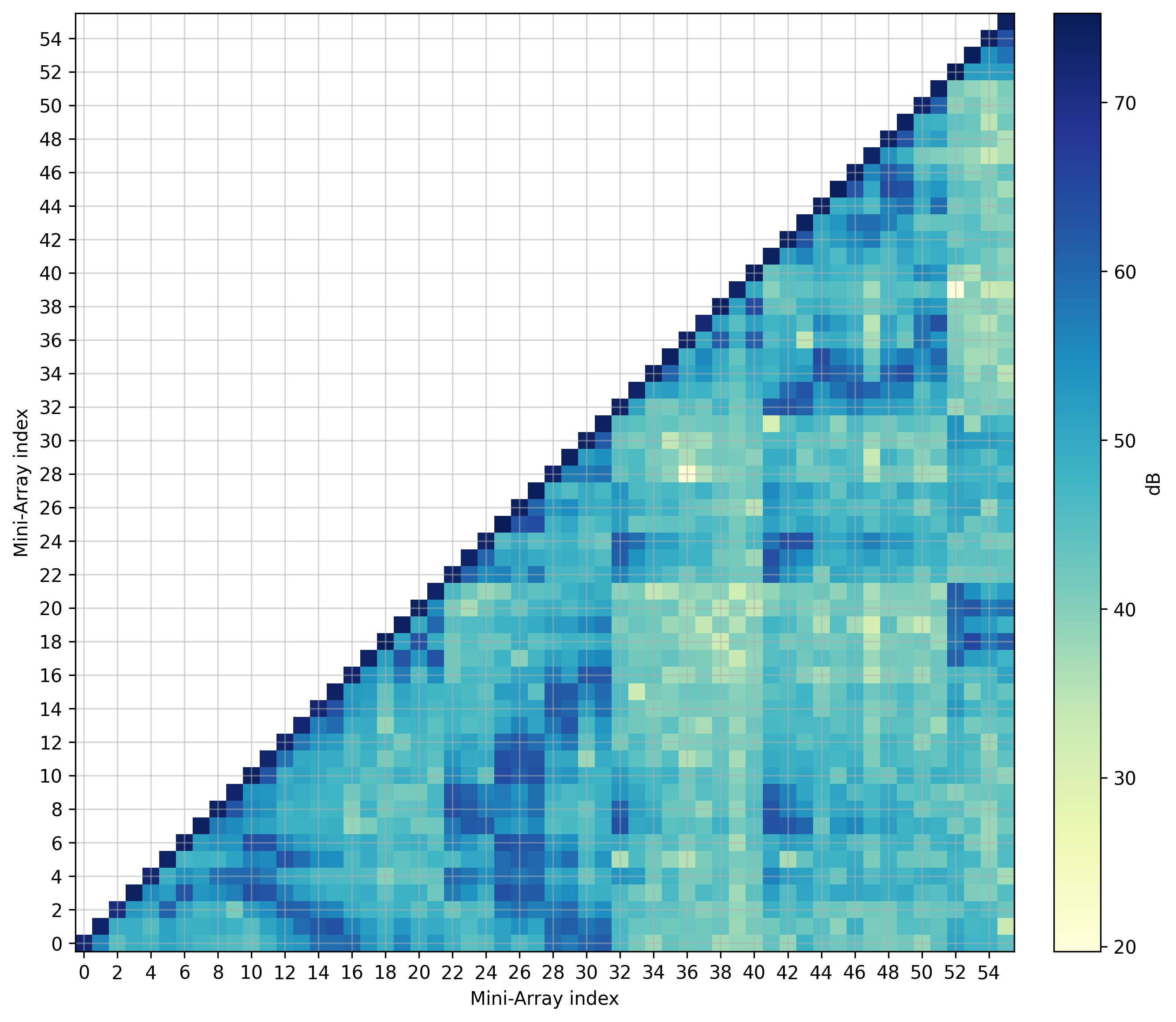
Cross-correlation matrix.

UV coverage from XST

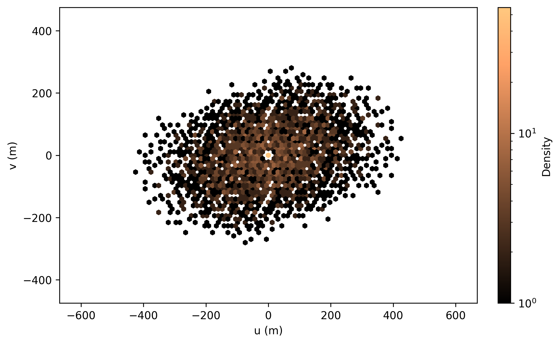
UV coverage (UV_Coverage) corresponding with the loded XST data can be easily displayed using its classmethod from_xst():

>>> from nenupy.io.xst import XST
>>> from nenupy.astro.uvw import UV_Coverage

>>> xst = XST(".../nenupy/tests/test_data/XST.fits")
>>> uvw = UV_Coverage.from_xst(xst)
>>> uvw.plot()

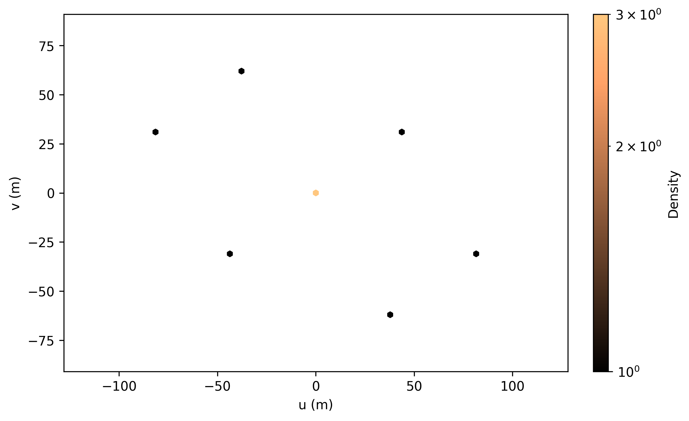
from_xst() takes also in input an XST_Slice, allowing for UV coverage display of selected visibilities:

>>> from nenupy.io.xst import XST
>>> from nenupy.astro.uvw import UV_Coverage

>>> xst = XST(".../nenupy/tests/test_data/XST.fits")
>>> xst_data = xst.get(miniarray_selection=np.array([0, 2, 10]))
>>> uvw = UV_Coverage.from_xst(xst_data)
>>> uvw.plot()

Beamforming from cross-correlations

XST contain recorded amplitude and phase data for each baseline involved in the observation. Hence their ability to be converted to beamformed statistics data (or BST) at will. This can in particular be done for any subset of Mini-Arrays in any pointing direction allowing for numerous potential array configurations available at once with a single XST observation, rather than performing a multi-pointing beam BST observation (at the cost of Sub-band number).

To demonstrate this property, the following considers a single NenuFAR observation data acquired simultaneously in BST and XST. The files are loaded using BST and XST:

>>> from nenupy.io.bst import BST
>>> from nenupy.io.xst import XST

>>> bst = BST("20191129_141900_BST.fits")
>>> xst = XST("20191129_141900_XST.fits")

>>> bst_data = bst.get(frequency_selection="==40.234375MHz", polarization="NW")

Beamforming the cross-correlation data is done using the get_beamform() method. The phasing direction must be provided. Hence, to compare the BST and XST data, a Pointing object is created directly from the metadata stored in the BST file using from_bst(). Similarly, the same Mini-Arrays and polarization are selected. Finally, the calibration table is specified (‘default’ value enables the calibration table used during the BST observation).

>>> from nenupy.astro.pointing import Pointing

>>> bf_cal = xst.get_beamform(
        pointing=Pointing.from_bst(bst, beam=0, analog=False),
        frequency_selection="==40.234375MHz",
        mini_arrays=bst.mini_arrays,
        polarization="NW",
        calibration="default"
    )

To compare the result, the selected BST data, the beamformed data using the calibration table and without using it (setting calibration="none") are displayed together:

>>> import matplotlib.pyplot as plt

>>> fig = plt.figure(figsize=(7, 4))
>>> plt.plot(bst_data.time.datetime, bst_data.value, label="BST data", linewidth=3)
>>> plt.plot(bf_uncal.time.datetime, bf_uncal.value, label="XST data uncalibrated", linewidth=1)
>>> plt.plot(bf_cal.time.datetime, bf_cal.value, label="XST data", linewidth=0.5, color="tab:red")
>>> plt.legend()
>>> plt.xlabel(f"Time (UTC from {bst_data.time[0].isot})")
>>> plt.ylabel("Amp")

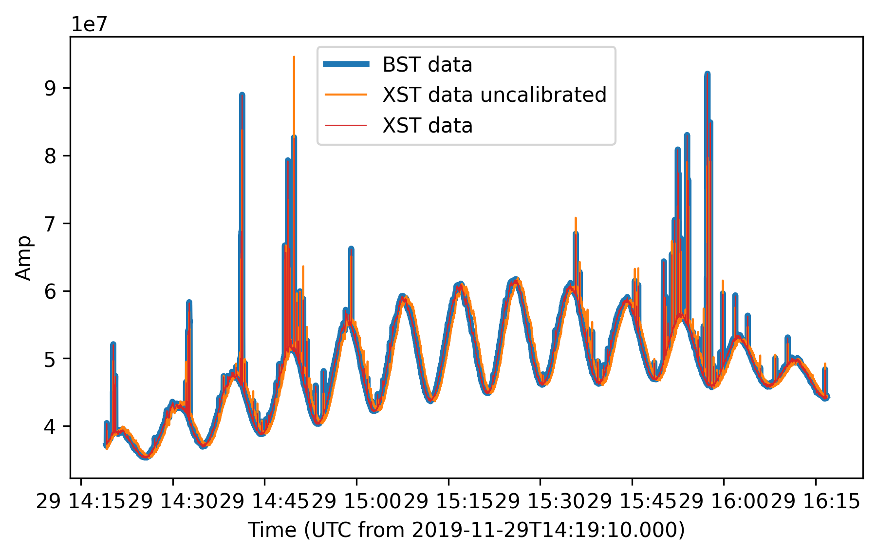
BST data versus time, against re-constructed beamformed data from XST (uncalibrated or calibrated with the default table used to obtain the BST). The blue (BST) and red (calibrated XST) curves are perfectly aligned as expected.

Image from XST

Once the XST data loaded (thanks to XST or NenufarTV), their selection (using for instance get_stokes()) outputs a XST_Slice instance. The method make_image() enables visibility inversion to make a ‘dirty image’ from the dataset in the HpxSky format. The method plot() is used to display the final image.

>>> import astropy.units as u
>>> from astropy.coordinates import SkyCoord

>>> xst_data = xst.get_stokes(
        stokes="I",
        miniarray_selection=None,
        frequency_selection=">=20MHz",
        time_selection=">=2019-11-19T15:15:00"
    )

>>> cyg_a = SkyCoord.from_name("Cyg A")

>>> im = xst_data.make_image(
        resolution=1*u.deg,
        fov_radius=20*u.deg,
        phase_center=cyg_a,
        stokes="I"
    )

>>> im[0, 0, 0].plot(
        center=cyg_a,
        radius=17*u.deg,
        colorbar_label="Stokes I (arb. units)",
        figsize=(8, 8),
    )

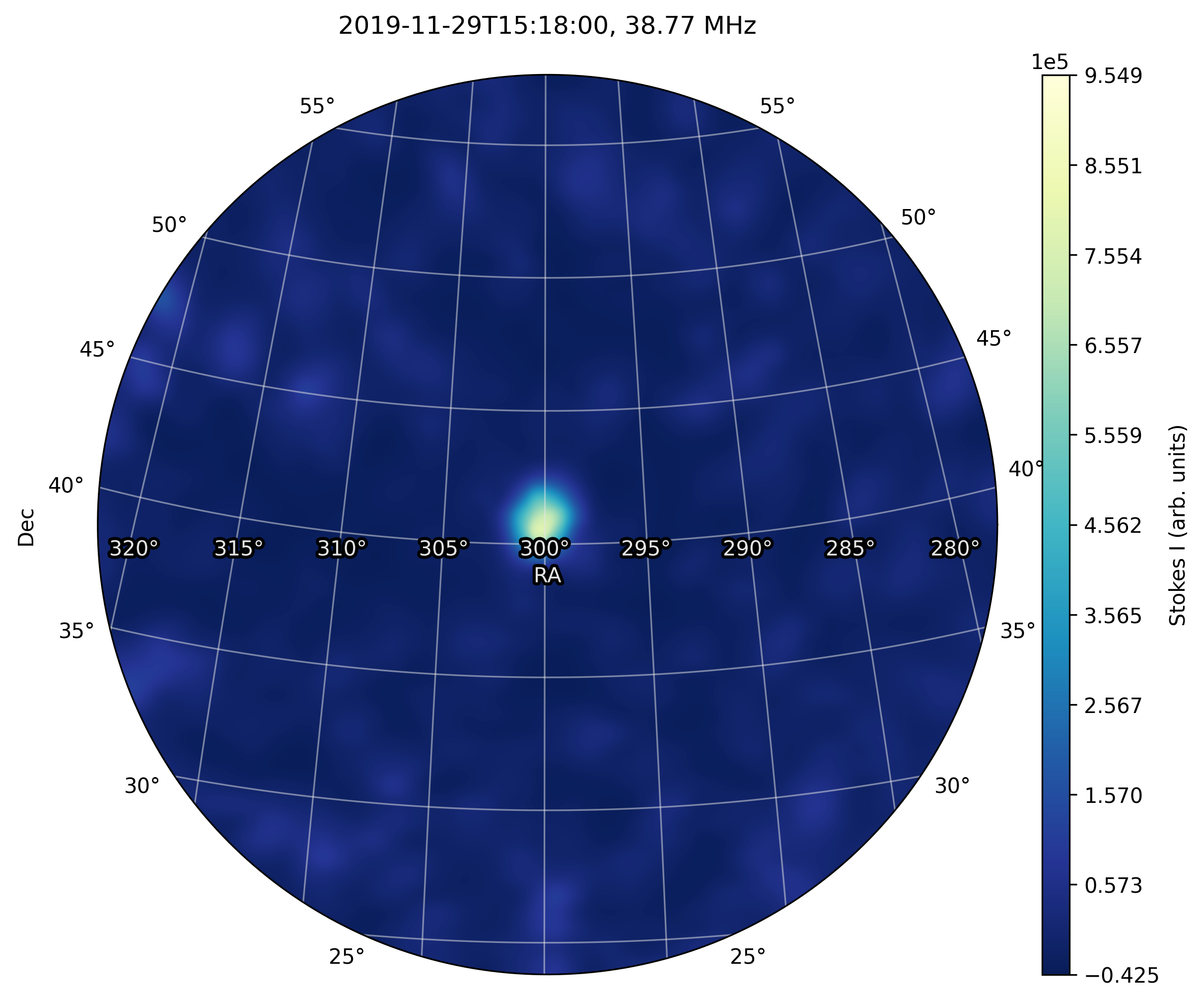
Cygnus A image obtained from XST data.

Near-field imprint from XST

Computing the near-field is pretty similar. Once the cross-correlations are selected using get_stokes(), make_nearfield() can be called to compute it. The returned values can be used to instanciate a TV_Nearfield object. The save_png() method is finally used to display the map:

>>> from nenupy.io.xst import TV_Nearfield
>>> import astropy.units as u

>>> xst_data = xst.get_stokes(
        stokes="I",
        miniarray_selection=None,
        frequency_selection=">=20MHz",
        time_selection="==2019-11-29T16:16:46.000"
    )

>>> radius = 400*u.m
>>> npix = 64
>>> nf, source_imprint = xst_data.make_nearfield(
        radius=radius,
        npix=npix,
        sources=["Cyg A", "Cas A", "Sun"]
    )

>>> nearfield = TV_Nearfield(
        nearfield=nf,
        source_imprints=source_imprint,
        npix=npix,
        time=xst_data.time[0],
        frequency=np.mean(xst_data.frequency),
        radius=radius,
        mini_arrays=xst_data.mini_arrays,
        stokes="I"
    )

>>> nearfield.save_png()

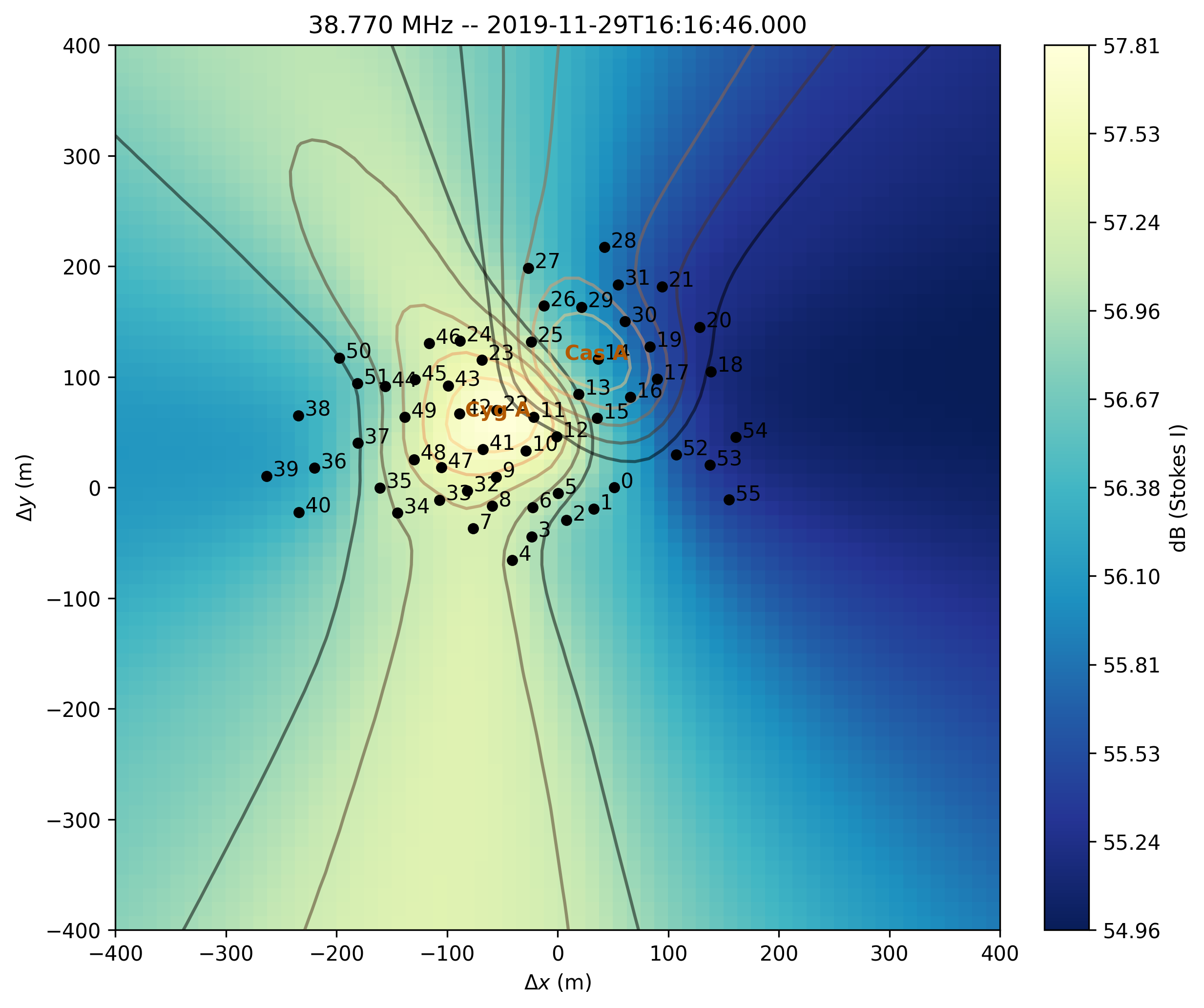
XST near-field.

NenuFAR TV

The class NenufarTV is exclusively used to read and load data corresponding with the NenuFAR-TV. Every 5 minutes, cross-correlations are taken along 16 sub-bands (for a total of around 3 MHz bandwidth), with a 10-sec time resolution. The data are stored in binary files that can be simply decoded by:

>>> from nenupy.io.xst import NenufarTV

>>> tv = NenufarTV("/path/to/nenufarTV.dat")

TV Image

Dedicated methods are attached to the NenufarTV class. The image can be directly computed using compute_nenufar_tv():

>>> from nenupy.io.xst import NenufarTV
>>> import astropy.units as u

>>> tv = NenufarTV("/path/to/nenufarTV.dat")

>>> tv_image = tv.compute_nenufar_tv(
        analog_pointing_file="<the_pointing_file.azana>",
        fov_radius=27 * u.deg,
        resolution=0.5 * u.deg,
        stokes="I"
    )
>>> tv_image.save_png()

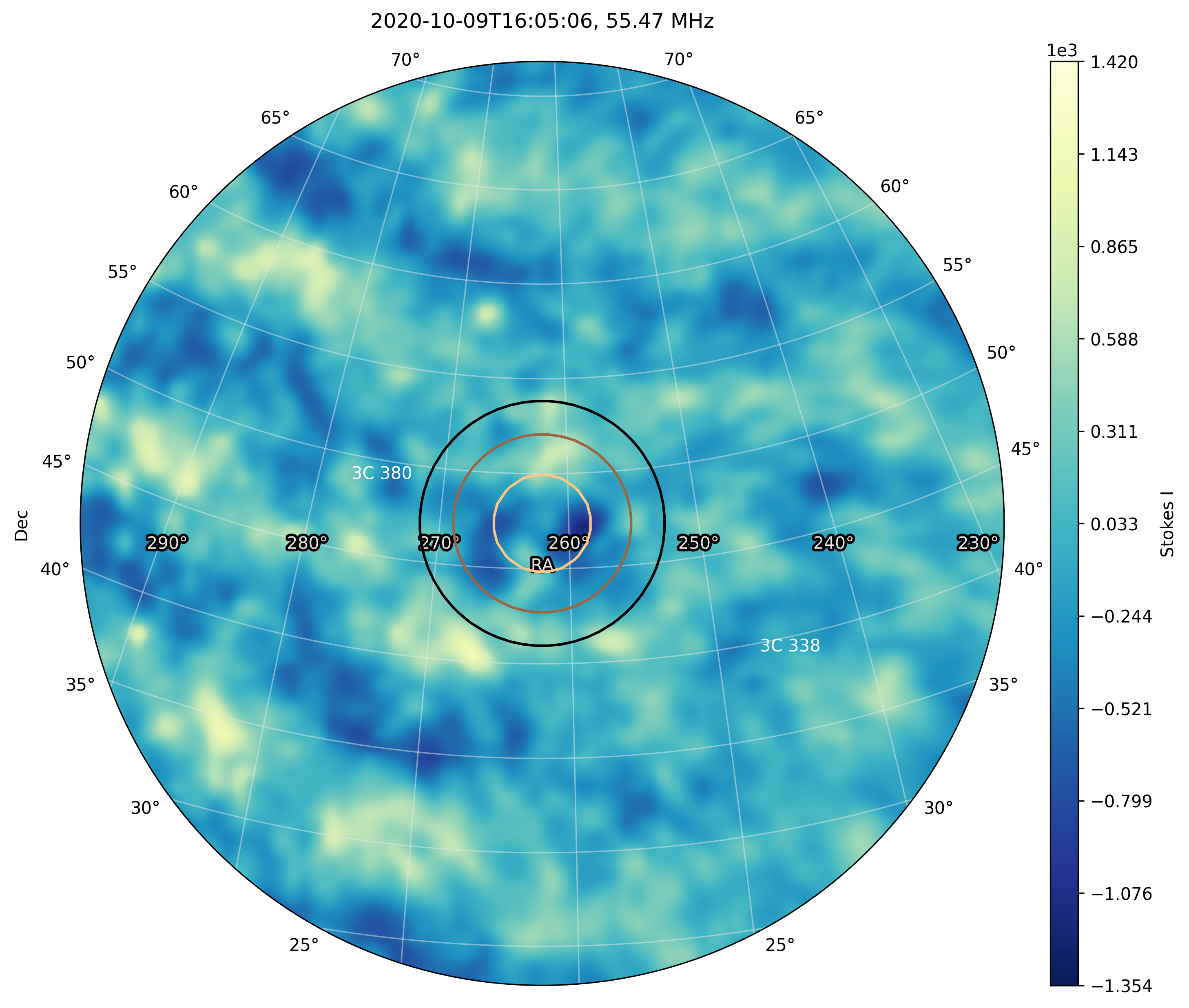
NenuFAR-TV image.

TV Near-field

The same is true for the near-field image, using the method compute_nearfield_tv():

>>> from nenupy.io.xst import NenufarTV
>>> import astropy.units as u

>>> tv = NenufarTV("/path/to/nenufarTV.dat")

>>> tv_nearfield = tv.compute_nearfield_tv(
        sources=["Cyg A", "Cas A"],
        stokes="I"
    )
>>> tv_nearfield.save_png()

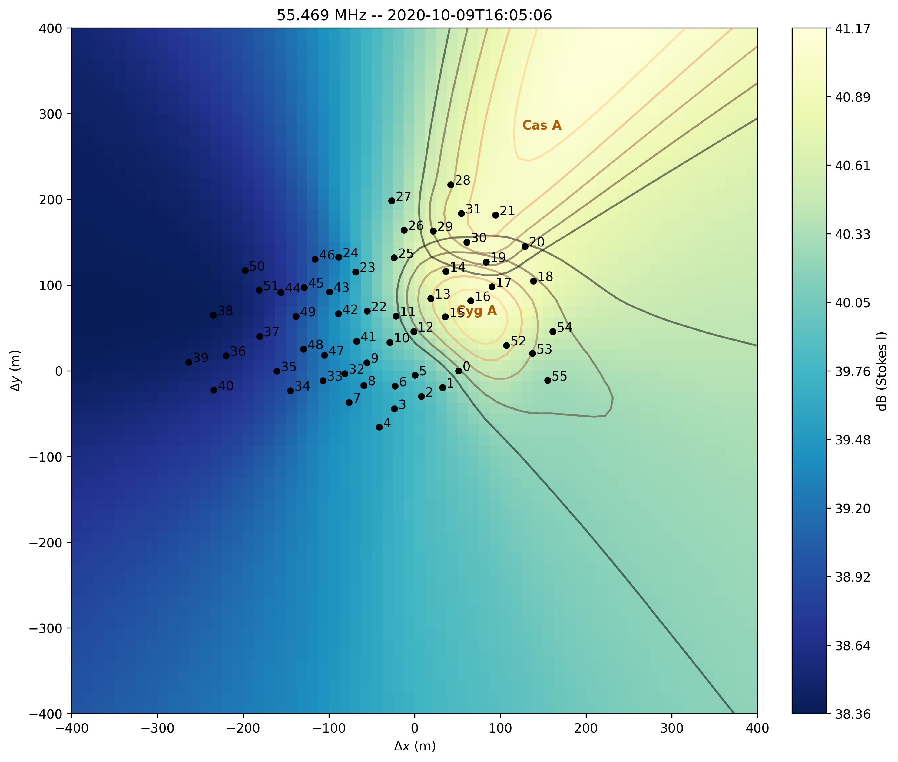
NenuFAR-TV near-field.