nenupy.io.tf_utils.mitigate_rfi_along_axis
- nenupy.io.tf_utils.mitigate_rfi_along_axis(data, axis=0, sigma_clip=2.0, polynomial_degree=4)[source]
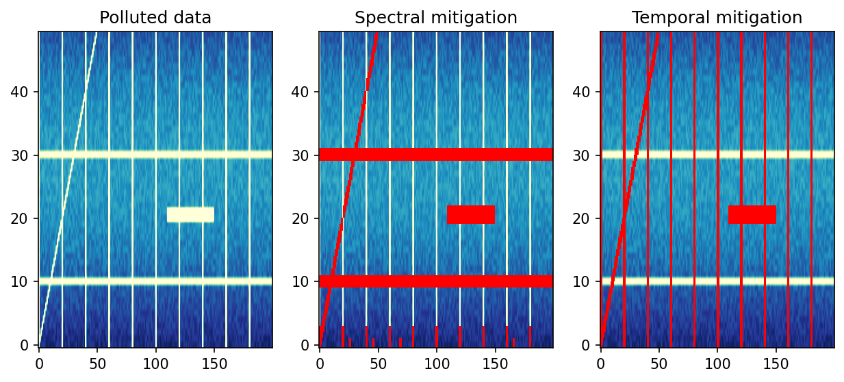
Perform sigma clipping along a given axis. Compute the median over one axis of a time-frequency dataset to obtain a background profile. Fit a polynomial function (of degree
polynomial_degree) to this profile, which will serve as a smooth background profile (the decimal logarithm of the data is used for fitting). Set every data points whose value is abovesigma_cliptimes the standard dedviation of the background profile to NaN values.- Parameters:
data (
Array) – The data to correct for RFI-like features, shaped like (time, frequency, (polarizations))axis (
int, optional) – Axis over which the median is computed, ifaxis=0the median will be done along the time dimension to obtain a spectral profile along which the RFI would be determined (and similarly foraxis=1), by default 0sigma_clip (
float, optional) – The factor above the background at which the data would be clipped, by default 2.polynomial_degree (
int, optional) – Degree of the polynomial function fitted to the time or spectral profile in order to smooth them, by default 4
- Returns:
The data whose outliers are set to NaN values.
- Return type:
Array- Raises:
Exception – If the input data is less than 2D.
IndexError – If the selected
axisis neither 0 or 1.
Examples
>>> from nenupy.io.tf_utils import mitigate_rfi_along_axis
>>> import numpy as np
>>> import matplotlib.pyplot as plt
>>> import matplotlib as mpl
>>> import dask.array as da

>>> polluted_data = 10**(4 + np.sin( np.pi * np.radians(np.arange(50))) + 0.5 * np.random.random((200, 50)))
>>> polluted_data[110:150, 20:22] += 10**9
>>> polluted_data[:, 10::20] += 10**7.5
>>> polluted_data[::20, :] += 10**10
>>> polluted_data[np.diag_indices(50)] += 10**9

>>> data_clean_axis_0 = mitigate_rfi_along_axis(
        data=da.from_array(polluted_data),
        axis=0,
        sigma_clip=3,
        polynomial_degree=5
    )
>>> data_clean_axis_1 = mitigate_rfi_along_axis(
        data=da.from_array(polluted_data),
        axis=1,
        sigma_clip=3,
        polynomial_degree=5
    )
>>> colors = mpl.colormaps.get_cmap("YlGnBu_r")
>>> colors.set_bad(color="red")

>>> vmin, vmax = 0, 8
>>> fig = plt.figure(figsize=(10, 4))
>>> axes = fig.subplots(nrows=1, ncols=3)
>>> axes[0].imshow(polluted_data.T, origin="lower", aspect="auto", cmap=colors, vmin=vmin, vmax=vmax)
>>> axes[0].set_title("Polluted data")
>>> axes[1].imshow(data_clean_axis_0.T, origin="lower", aspect="auto", cmap=colors, vmin=vmin, vmax=vmax)
>>> axes[1].set_title("Spectral mitigation")
>>> axes[2].imshow(data_clean_axis_1.T, origin="lower", aspect="auto", cmap=colors, vmin=vmin, vmax=vmax)
>>> axes[2].set_title("Temporal mitigation")