nenupy.io.xst.XST_Slice
- class nenupy.io.xst.XST_Slice(mini_arrays, time, frequency, value, phase_center=None)[source]
Bases:
objectClass to handle the result of selection upon XST-like data.
See also
- __init__(mini_arrays, time, frequency, value, phase_center=None)[source]
Generate an instance of
XST_Slice.- Parameters:
mini_arrays (
ndarray) – NenuFAR Mini-Arrays involved in the data selectiontime (
Time) – Time description of the selected datasetfrequency (
Quantity) – Frequency description of the selected datasetvalue (
ndarray) – Data selection values, it should have the shape \((n_{\rm \nu},\, n_{t},\, n_{\rm bl})\) where \(n_{\rm \nu}\), \(n_{t}\) and \(n_{\rm bl}=n_{\rm ant}(n_{\rm ant} - 1)/2 + n_{\rm ant}\) are respectively the number of frequency and time samples, and the number of baselinesphase_center (
SkyCoord) – Phase center of the visibility selection (in ICRS), by defaultNone(i.e., zenith)
Methods
__init__(mini_arrays, time, frequency, value)Generate an instance of
XST_Slice.make_image([resolution, fov_radius, ...])Perform an inversion of the visibilities to get an image.
make_nearfield([radius, npix, sources])Computes the near-field image from the cross-correlation statistics data \(\mathcal{V}\).
plot_correlaton_matrix([...])Plot the XST cross-correlation matrix.
rephase_visibilities(phase_center[, uvw])Rephase the XST visibilities towards a new phase center.
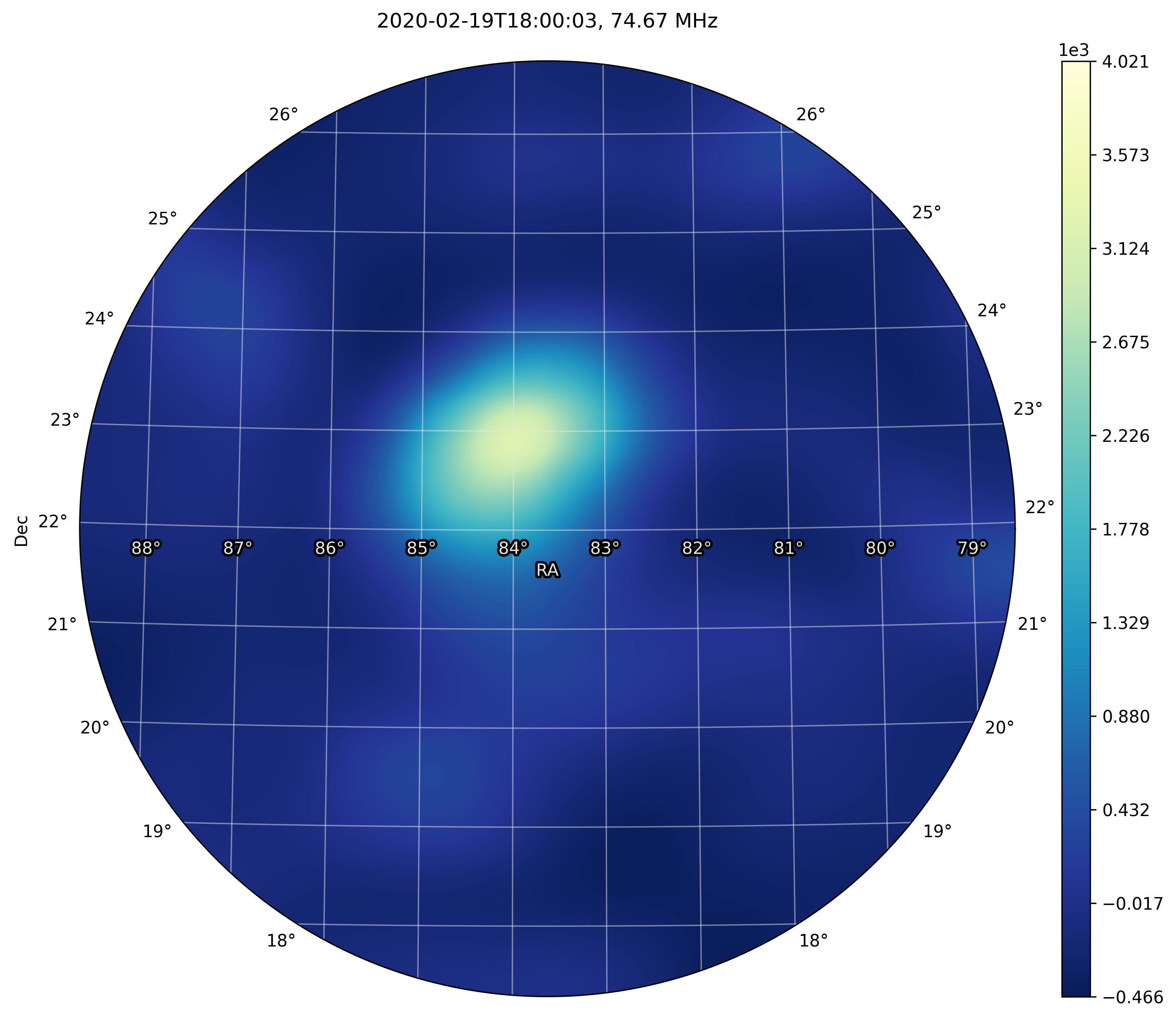
- make_image(resolution=<Quantity 1. deg>, fov_radius=<Quantity 25. deg>, phase_center=None, stokes='I')[source]
Perform an inversion of the visibilities to get an image.
A Discrete Fourier Transform is applied, based on the Fourier Transform relationship between the sky brightness distribution \(\mathcal{I}(l,m,n)\) and the NenuFAR response (complex visibilities) \(\mathcal{V}(u,v,w)\):
\[\mathcal{I}(l, m, n) = \int \left\langle \mathcal{V}(u, v, w) \right\rangle_{t, \nu} e^{-2\pi i (ul + vm + wn)}\,du\, dv\, dw ,\]where \((u, v, w)\) are coordinates expressed in \(\lambda\) units, \((l,m,n)\) are image coordinates (taken as an HEALPix image by default using
HpxSky).- Parameters:
resolution (
Quantity, optional) – Image HEALPix resolution (seeHpxSky), by default 1 degreefov_radius (
Quantity, optional) – Field of View radius that will apply a selection on the image plane before computing the pixel values, by default 25 degreesphase_center (
SkyCoord, optional) – Center of the field of view, by defaultNone(i.e., local zenith)stokes (
str, optional) – Stokes parameter description of what contain thevaluethat will be passed toHpxSky(there is no computation dependency upon this paramater here), by default “I”
- Returns:
The image
- Return type:
Example
>>> from nenupy.io.xst import XST
>>> from astropy.coordinates import SkyCoord
>>> import astropy.units as u

>>> xst = XST(".../nenupy/tests/test_data/XST.fits")
>>> xx_data = xst.get(polarization="XX")
>>> tau_a = SkyCoord.from_name("Tau A")
>>> im = xx_data.make_image(
        resolution=1*u.deg,
        fov_radius=10*u.deg,
        phase_center=tau_a,
        stokes="XX"
    )

>>> im[0, 0, 0].plot(center=tau_a, radius=5*u.deg)
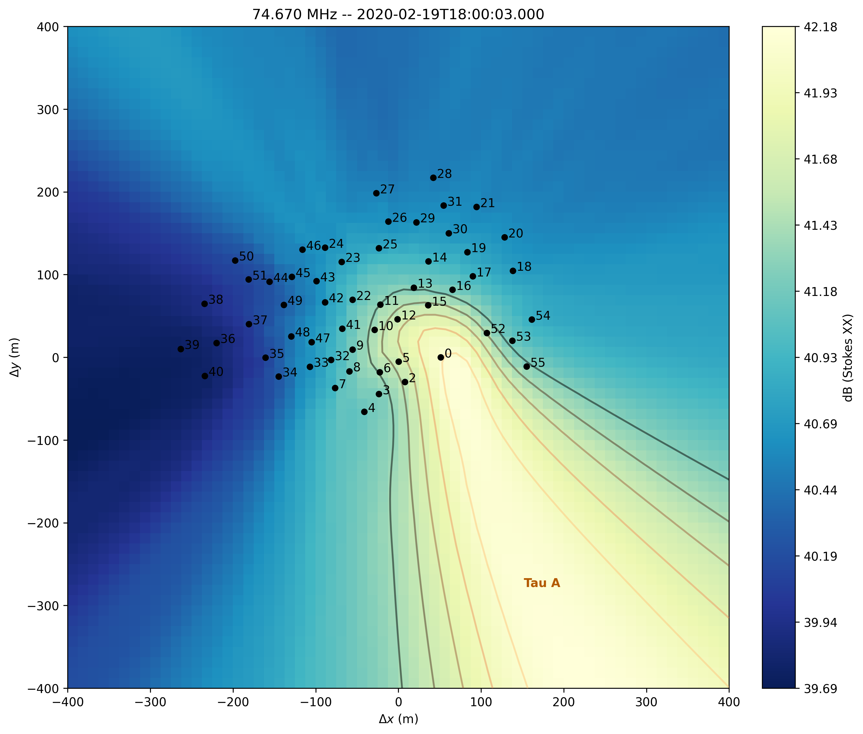
- make_nearfield(radius=<Quantity 400. m>, npix=64, sources=[])[source]
Computes the near-field image from the cross-correlation statistics data \(\mathcal{V}\).
The distances between each Mini-Array \({\rm MA}_i\) and the ground positions \(\Delta\) is:
\[d_{\rm{MA}_i} (x, y) = \sqrt{ ({\rm MA}_{i, x} - \Delta_x)^2 + ({\rm MA}_{i, y} - \Delta_y)^2 + \left( {\rm MA}_{i, z} - \sum_j \frac{{\rm MA}_{j, z}}{n_{\rm MA}} - 1 \right)^2 }\]Then, the near-field image \(n_f\) can be retrieved as follows (\(k\) and \(l\) being two distinct Mini-Arrays):
\[n_f (x, y) = \sum_{k, l} \left| \sum_{\nu} \langle \mathcal{V}_{\nu, k, l}(t) \rangle_t e^{2 \pi i \left( d_{{\rm MA}_k} - d_{{\rm MA}_l} \right) (x, y) \frac{\nu}{c}} \right|\]Notes
To simulate astrophysical source of brightness \(\mathcal{B}\) footprint on the near-field, its visibility per baseline of Mini-Arrays \(k\) and \(l\) are computed as:
\[\mathcal{V}_{{\rm simu}, k, l} = \mathcal{B} e^{2 \pi i \left( \mathbf{r}_k - \mathbf{r}_l \right) \cdot \mathbf{u} \frac{\nu}{c}}\]with \(\mathbf{r}\) the ENU position of the Mini-Arrays, \(\mathbf{u} = \left( \cos(\theta) \sin(\phi), \cos(\theta) \cos(\phi), sin(\theta) \right)\) the ground projection vector (in East-North-Up coordinates), (\(\phi\) and \(\theta\) are the source horizontal coordinates azimuth and elevation respectively).
- Parameters:
radius (
Quantity, optional) – Radius of the ground image, by default 400 mnpix (
int, optional) – Number of pixels of the image size, by default 64.sources (List[
int], optional) – List of source names for which their near-field footprint may be computed (only sources above 10 deg elevation will be considered), source names are resolved using Simbad throughfrom_name()withinFixedTarget, Solar System object names are also valid (and called throughSolarSystemTarget), by default []
- Returns:
Tuple of near-field image (of shape
(npix, npix)) and a dictionnary containing all source footprints (of the same shapes)- Return type:
Example
>>> from nenupy.io.xst import XST

>>> xst = XST(".../nenupy/tests/test_data/XST.fits")
>>> xx_data = xst.get(polarization="XX")
>>> nearfield, src_dict = xx_data.make_nearfield(
        radius=400*u.m,
        npix=64,
        sources=["Tau A"]
    )
One can further plot the nearfield map:
>>> from nenupy.io.xst import TV_Nearfield

>>> tv_nf = TV_Nearfield(
        nearfield=nearfield,
        source_imprints=src_dict,
        npix=nearfield.shape[0],
        time=xst.time[0],
        frequency=xst.frequencies[0],
        radius=400*u.m,
        mini_arrays=xst.mini_arrays,
        stokes="XX",
    )
>>> tv_nf.save_png(figname="")
Added in version 1.1.0.
- plot_correlaton_matrix(mask_autocorrelations=False, figsize=(10, 10), decibel=True, cmap='YlGnBu', vmin=None, vmax=None, cbar_label=None, title=None, figname=None)[source]
Plot the XST cross-correlation matrix. All visibilities are plotted against their Mini-Array indices. The absolute of their average over their available time and frequency samples is displayed.
- Parameters:
mask_autocorrelations (
bool, optional) – Mask the auto-correlation diagonal, by defaultFalsefigsize (Tuple[
int,int], optional) – Size of the figure, by default (10, 10)decibel (
bool, optional) – Set the scale of the data displayed to dB (i.e., \({\rm dB} = 10 \log_{10}({\rm data})\)), by default Truecmap (
str, optional) – Color map used to represent the data, by default “YlGnBu”vmin (
float, optional) – Minimal value displayed, by defaultNone(i.e., overall minimal value)vmax (
float, optional) – Maximal value displayed, by defaultNone(i.e., overall maximal value)cbar_label (
str, optional) – Label of the color bar, by defaultNonefigname (
str, optional) – Name of the figure, if given the figure will be saved, by defaultNone
Example
>>> from nenupy.io.xst import XST

>>> xst = XST("/path/to/XST.fits")
>>> data = xst.get(...) # data selection that generate a XST_Slice
>>> data.plot_correlaton_matrix()
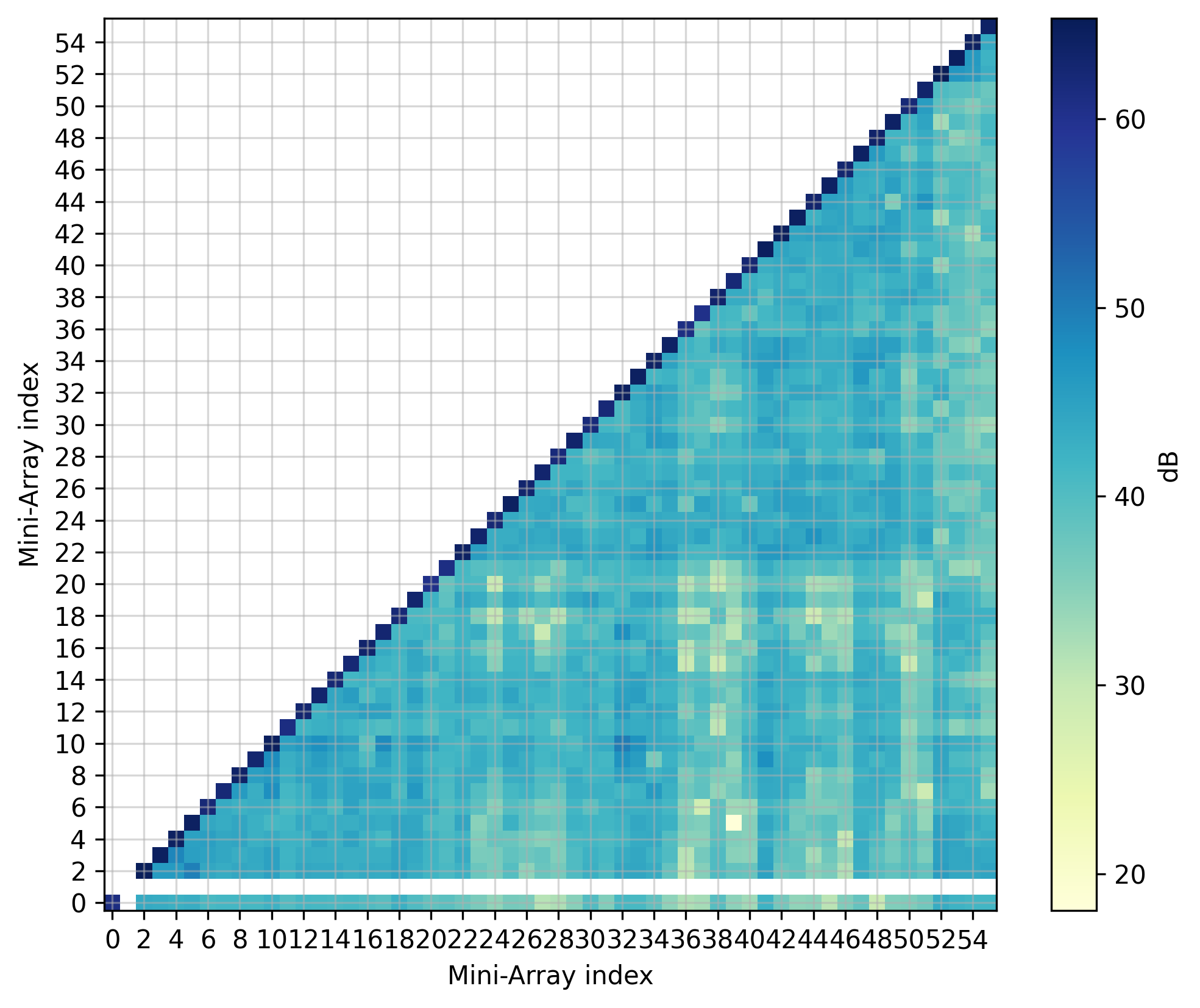
Cross-correlation matrix, the Mini-Array #1 was flagged.
- rephase_visibilities(phase_center, uvw=None)[source]
Rephase the XST visibilities towards a new phase center. By default, XST visibilities are phased at the local zenith. This method applies two rotations: one to reset the visibilities to the celestial frame origin and a second to phase towards the desired phase center.
- Parameters:
phase_center (
SkyCoord) – New phase center.uvw (
ndarray) – UVW coordinates in meters of the input array, see alsocompute_uvw(), by defaultNone(i.e., the method automatically computes the cooridnates)
- Returns:
Re-phased visibilities, rotated UVW coordinates
- Return type:
Example
>>> from nenupy.io.xst import XST
>>> from astropy.coordinates import SkyCoord

>>> xst = XST("/path/to/XST.fits")
>>> xx_data = xst.get(polarization="XX")
>>> cyg_a = SkyCoord.from_name("Cyg A")
>>> xx_data_rephased, uvw_rephased = xx_data.rephase_visibilities(cyg_a)