nenupy.io.tf_utils.de_faraday_data

nenupy.io.tf_utils.de_faraday_data(data, frequency, rotation_measure)[source]

Correct the data from Faraday Rotation effect.

Linearly polarized light travelling through a magnetized plasma is subject to a rotation of its polarization direction due to charged particles (mostly dominated by electrons) reacting to and influencing differentially the magnetic field components of the electromagnetic radiation.

This function computes the chromatic Faraday rotation angle to correct for \(\theta (\nu)\) with faraday_angle(), given the rotation_measure of the intervening plasma. It is equivalent as computing \(\Delta \theta = | \theta (\nu_{\rm ref}) - \theta (\nu) |\), i.e., the difference of rotation angle where every frequency is compared to an ‘infinite’ frequency (since \(\theta \propto \nu^{-2}\)).

\[\mathbf{d}_{\rm corrected}(t, \nu) = \mathbf{R}(\nu) \mathbf{d}(t, \nu) \mathbf{R}(\nu)^\top,\]

where

\[\begin{split}\mathbf{R}(\nu) = \begin{pmatrix} \cos \theta (\nu) & - \sin \theta (\nu) \\ \sin \theta (\nu) & \cos \theta (\nu) \end{pmatrix}\end{split}\]

is the Faraday rotation matrix and

\[\begin{split}\mathbf{d}(t, \nu) = \begin{pmatrix} e_{\rm x}\overline{e_{\rm x}} & e_{\rm x}\overline{e_{\rm y}} \\ e_{\rm y}\overline{e_{\rm x}} & e_{\rm y}\overline{e_{\rm y}} \end{pmatrix}(t, \nu),\end{split}\]

and similarly \(\mathbf{d}_{\rm corrected}\) are the data and corrected data returned by this function, shaped as Jones matrices of the signal. \(t\) and \(\nu\) are the time and frequency.

Parameters:

frequency (Quantity) – Light frequency (in units equivalent to MHz).
data (ndarray) – Data in Jones format to be corrected. It needs to be shaped like (time, frequency, 2, 2)
rotation_measure (Quantity) – Rotation measure (in units equivalent to rad/m2).

Returns:

Faraday rotation corrected data.

Return type:

ndarray

Raises:

Exception – Raised if the data dimensions do not meet the requirements.

Examples

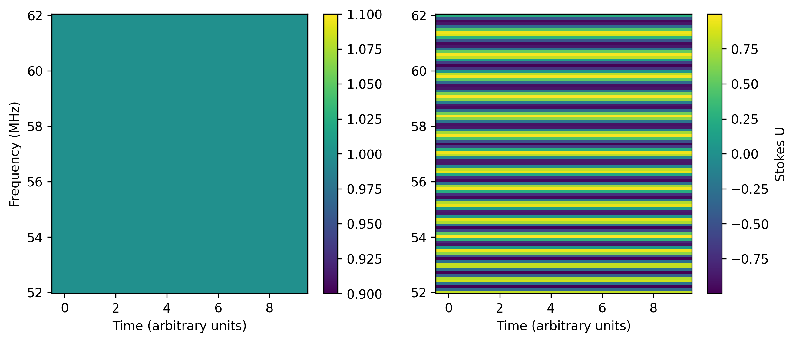
>>> import numpy as np
>>> import astropy.units as u
>>> import matplotlib.pyplot as plt
>>> from nenupy.io.tf_utils import de_faraday_data

>>> times = np.arange(10)
>>> frequencies = np.linspace(52, 62, 100) * u.MHz
>>> linearly_polarized_light = 0.5 * np.array([[1, 1], [1, 1]]) # 45 deg
>>> linearly_polarized_light = np.tile(linearly_polarized_light, (times.size, frequencies.size, 1, 1))
>>> stokes_u = linearly_polarized_light[..., 0, 1] * 2
>>> faraday_rotated_light = de_faraday_data(
        data=linearly_polarized_light,
        frequency=frequencies,
        rotation_measure=5 * u.rad / u.m**2
    )
>>> faraday_stokes_u = faraday_rotated_light[..., 0, 1] * 2

>>> fig = plt.figure(figsize=(10, 4))
>>> axes = fig.subplots(nrows=1, ncols=2)
>>> im_0 = axes[0].pcolormesh(times, frequencies.to_value(u.MHz), stokes_u.T)
>>> im_1 = axes[1].pcolormesh(times, frequencies.to_value(u.MHz), faraday_stokes_u.T)
>>> cbar_0 = plt.colorbar(im_0)
>>> cbar_1 = plt.colorbar(im_1)
>>> cbar_1.set_label(r"Stokes U")
>>> axes[0].set_ylabel("Frequency (MHz)")
>>> axes[0].set_xlabel("Time (arbitrary units)")
>>> axes[1].set_xlabel("Time (arbitrary units)")