nenupy.io.tf_utils.flatten_subband
- nenupy.io.tf_utils.flatten_subband(data, channels, smooth_frequency_profile=False)[source]
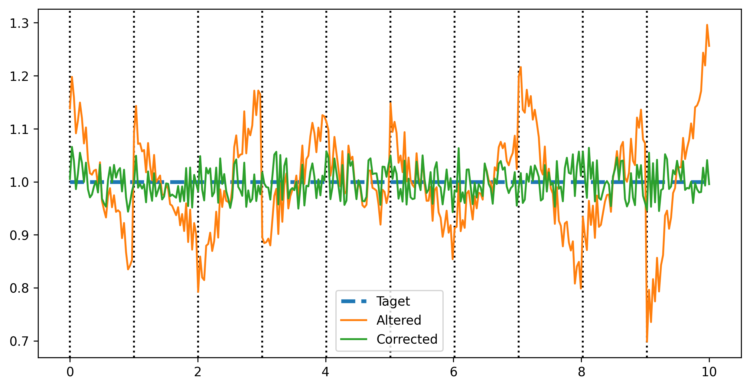
Correct each subband if their levels is distributed like a sawtooth. Sometimes, in particular for strong sources, the subbands adopt a strange behavior (an example is shown in
flatten_subband()). This function aims at correcting this effect.For a given subband:
The median frequency profile is computed over the whole data time selection
Affine function is computed based on two points taken as the medians of both half profiles of the subband
This function is normalized by the median of the subband total profile
The corrected subband is the original subband divided by this normalized linear profile
- Parameters:
- Returns:
The corrected data, where the subbands are flattened.
- Return type:
- Raises:
ValueError – Raised if the
datadimension 1, assumed to be the frequency, does not matchchannels.
Examples
>>> from nenupy.io.tf_utils import flatten_subband
>>> import numpy as np
>>> import matplotlib.pyplot as plt

>>> n_channels = 32
>>> n_subbands = 10

>>> rng = np.random.default_rng(12345)
>>> coeffs = rng.uniform(-0.1, 0.1, size=n_subbands)

>>> x_data = np.linspace(0, 10, n_channels * n_subbands)
>>> y_data = np.ones(x_data.size) # Idel data are flat
>>> saw_pattern = (coeffs[:, None]*np.linspace(-3, 3, n_channels) )[None, :]
>>> noise = rng.uniform(-0.05, 0.05, x_data.size)
>>> y_data_altered = (y_data.reshape((n_subbands, n_channels)) + saw_pattern).ravel() + noise

>>> y_data_corrected = flatten_subband(
        data=y_data_altered.reshape(1, y_data_altered.size, 1, 1),
        channels=n_channels
    )

>>> fig = plt.figure(figsize=(10, 5))
>>> for sb in range(n_subbands):
>>>     plt.axvline(x_data[sb*n_channels], color="black", linestyle=":")
>>> plt.plot(x_data, y_data, label="Original", linewidth=3, linestyle="--")
>>> plt.plot(x_data, y_data_altered, label="Altered")
>>> plt.plot(x_data, y_data_corrected[0, :, 0, 0], label="Corrected")
>>> plt.legend()